Fluorescent Afterburner

Once you’ve got the basic parameters working, you can start playing with their variation as well as adding new ones.
Particles offer a great deal of the features and parameters to suit just about all your needs. However, as a beginner you’ll most likely end up fiddling with pretty much all of them before getting the result your after (or simlpy giving up because you’re no where near it). Just because you have a parameter at your disposal doesn’t mean it will add anything to your current setup or that you should use it. On the contrary, keeping it simple will drastically increase your chances of succeeding.

Start by pressing [4] to switch to the simulation toolbar. From the Create > Particles > From Primitive menu, choose From Disk. Click on the lock icon in the Particles PPG to ensure it will stay in place trough out the procedure and scroll down to the PType > Overview section. The first thing you obviously will need to do is changing the color to cool blueish tone. Click the animation icon (the green dot) to set a keyframe. Go to frame 100, make the blue slightly brighter and set the alpha to 0 (zero). Set a new keyframe. In the Animation Reference section, change the RGB and Alpha to Age %. The Max Life will control the length of your afterburner. Set it to about 0.3 and increase the Size to about 4. Go to the Particle_Billboard > Rendering Properties and check the Rotation Follow Velocity checkbox. In the Effects section, set the Burn to 1 to create a bright intense core in the combustion. You don’t want the particles to be affected by the lighting in your scene, so switch to the Shading Properties tab and uncheck the Apply Shading checkbox.

The afterburner is starting to come together but the shape still look slightly of. Go to the Particle_Shape > Shape and change the Type to Beam Pattern and set the Width to about 0.035. The last thing you’ll need to is to increase the number of particles and their speed, so scroll back to the Emission > Overview. Set the Rate to about 4000 and the Speed to 35. Remove any highly flammable material, hit the play button and your ready to take of into space.

The project files used in this tutorial can be found at:
http://www.Redi-Vivus.com/Caffeineabuse/Fluorescent_Afterburner.zip

For an even greater control of the shape of your afterburner you can make use of sprites instead of the Beam Pattern shape.
Quick tip
Switching the background color in your viewports to black (in the Camera icon menu in your viewport) and the Display Type to textured will limit the need to render each and every frame to se the effect of your settings.

Read the full post>>

Sound Vibration

Step 1
Install the addon
Start by installing the Sound2Curve addon by Guy Rabiller, which can be found at http://grabiller.3dvf.net/site/content/addons_s2c_eng.html. This script creates an fcurve based on an audio file (.wav) In case you don’t have any audio file to actually sync with or just want the random motion, you can use the random fcurve script instead, which can be found in the netview





















Step 2
Deforming the geometry
Load the scene speaker.scn and run the Sound2Curve script (se the website for further information). There’s numerous ways to deform the geometry of the speaker. In this scenario will make use of the volume deformer since it, apart from being easy to control, gives a nice falloff to the deformation. While everything is already setup for you in the scene, try playing with the settings to customize the effect for your specific needs.
Step 3
Copy the animation
Select the Null created by the Sound2Curve script and press [0] (zero) to open the Animation Editor. In the animation tree, right click on the posy and choose copy animation. Now, select the Volume_deform object (you might need to change the filter in the AE to see none animated parameters), right click on the posz and choose paste animation. Now use the region and/or the HLE too in the AE to scale and modify the fcurve to better suit your current environment.

The project files used in this tutorial can be found at:http://www.Redi-Vivus.com/Caffeineabuse/Sound_Vibration.zip

Read the full post>>

Bowling Alley Timewarp

The basic idea of bowling is rather simple; throw a big heavy ball down a rigorous polished wooden floor and keep your fingers crossed that you’ll knock over at least one of the oddly shaped thingies at the end of the lane. Obviously there’s a lot more to the game that the above and the bizarre shoes, so in order for us to setup our alley truthfully we might as well have a crash course in the art of bowling as we go trough the various steps on the following pages.

Even if there are no more than eleven objects to animate, the ball and ten pins, it will still be a rather tedious task animating them all by hand due to the way they are supposed to interact with each other. Unless were aiming for some truly extraordinary motions for the pins (which can be achieved by additional keyframe animation), XSI rigid body dynamics (RBD) will be right up our alley. Consequently we’ll inevitable be facing the constant reoccurring question about scale and Softimage Units. The truth is that a Softimage Unit equals exactly anything you want it to. Whether it’s an inch, centimeter or a mile is arbitrary, and won’t make a difference as long as you know what it’s representing in your current environment. However, for the values used in the simulation to make any sense at all, it’s important to note that they by default are based on the relation of one unit equals 10 centimeter.

The second part of the problem requires a bit of further manipulation, which will take place in the animation mixer. While we theoretical can animate the change of time/speed in the animation by hand, it would have us facing a big problem since we’re driving the all the motions with RBD. Decreasing the forces and the speed of the ball could indeed give the desired impression of slow-motion but will unavoidable also alter how the objects interact. If we, for instance, reduce the speed of the ball under a certain limit it won’t have enough energy to knock down any of the pins. Instead we’ll run the simulation at full speed, cash the position and orientation of each object at every frame as a clip in the animation mixer. Once that is done we can easily animate the speed of the clip (known as time warp) and thus having full freedom of the camera motion.

The project files used in this tutorial can be found at:
http://www.Redi-Vivus.com/Caffeineabuse/BowlingAlley.zip

Stage one The alley
Step 1
Start by loading the scene bowling_alley.scn from the CD. Apart from the refreshments, the scene contains all the ingredients needed for a successful night of bowling. The first thing we need to do is to setup the physical rules, which are to control the interaction between the scene components.
Step 2
Press [4] to switch to the Simulate Toolbar. The bowling lane itself shouldn’t be affected by the dynamics in the scene (such as the gravity), so for that reason we’ll turn it in to passive rigid body. This is done by selecting the lane object and from the Create > Rigid Body menu choose Passive Rigid Body. Leave the default settings as they are and close the PPG.
Step 3
Both the ball and the pins on the other hand, should all be used to act and react with each other. Select all of them (11 objects in total) and from the Create > Rigid Body menu choose Active Rigid Body. We’ll be working on the settings separately so to ensure optimal interaction check the Mute checkbox to temporarily exclude them from the simulation and close the PPG.

Stage two The ball
Step 4
Select the ball alone and from the Modify > Rigid Body menu click Edit Rigid Body to open its PPG. Bowling regulations prohibits balls from weighting more 7.26 kg (and circumference grater that 68.6 cm). Under the Inertial Properties, enter 6 as the Mass and we’ll stay well under the limit. You can always return and change any of these values later on to fine-tune or experiment with the outcome.






















Step 5
Scroll down to the Rigid Body Properties and uncheck the Mute checkbox. By default the collision type is set to Bounding Box, which evidently won’t produce very realistic results for our ball. So change the type to Bounding Sphere instead. The next step is to set how and when the ball will start losing its energy.




















Step 6
The Elasticity determines how much of the energy that will be lost (or gained) when the ball collides with another object whereas the Friction determines how much will be lost as it rolls along the surface of the lane. Set the Elasticity to about 0.5 and the Friction to 0.25. These parameters are obviously affected by the same values of the other objects in the simulation, so you might want to return and fine-tune them later on.

Stage Three Preparing the hook
Step 7
Before start working with motions we’ll need to add gravity. Any force added to the scene is automatically assigned to all RBD objects in the environment. From the Get > Force menu click Gravity. As we’ve constructed out objects in the “correct” scale (refer to the introductory text), we can just leave the Amplitude settings as they are.
Step 8
Due to the layout of the pins it’s not possible to knock all of them down with the ball alone, but one has to rely on the pins hitting each other. Most inexperienced bowlers throw the ball in a straight line, aiming directly at the firs pin, whereas the more experienced player usually have developed a hook. Given we’re well on the route of becoming skilled bowlers we might as well do it the hip way.
Step 9
A neat feature in XSI is the ability to use Ghosting, which is available even when working with RBD simulations. Press [6] to open the Layer Control Window. Click the empty checkbox at the very right to activate Ghosting for all objects in the layer. This enables us to se the position of the ball throughout its animation without actually running the simulation.

Stage Four Scoring a strike


Step 10
Return to the Dynamics PPG of the ball and under the Dynamics Initial State switch to the Velocity tab. Since there’s currently no animation assigned the ball we need to give it some initial energy. Enter –70 as the LinVelZ. With some quick mental calculation we’ll see that a value of 70 actually means the ball will travel just over 25 km per hour, 70 units equals 7 meters (per second) times 3600 seconds.
Step 11
To achieve the curved path we’re striving for, we’ll also need to throw the ball at a slight angle rather that straight down the lane. Set the LinVelX to about 5.5. Now the ball obviously runs way out of out bounds. To fix this we’ll need to make it spin, there by forcing it back towards the pins as it travels down the lane.
Step 12
The amount of spin needed depends on the strength of the LinVelx and LinVelZ. The plan is to make the ball hit the pins between pin one and three, assuming your aiming for a strike. Under the Angular section, enter about 1350 as the AngVelZ value as this should do the job nicely. Play with the setting till you you’re happy with the shape of the path.

Stage five The pins
Step 13
Before start working with the parameters for the pins it’s recommended to turn off the Ghosting, as this can otherwise slow down the system considerably. Select all ten pins and from the Modify > Rigid Body menu click Edit Rigid Body. These are still excluded from simulation so start with un-checking the Mute checkbox under the Rigid Body Properties.
Step 14
The Bounding Box collision type won’t work very well once the pins fall over so let’s change it Bounding Capsule. Although there is an Actual Shape available as the collision type, you’ll run a great risk of unpredictable result and even stability issues when using it (in XSI ver 4.2). So unless truly needed, I recommend you not to use it.























Step 15
A high Elasticity value, such as one (above one will add energy at each collision), will give you lots of bouncing whereas a low value will bring them to a rest quickly. Set the Elasticity to 1 and the Friction to 0.25. To add some more characteristic to their motion, set the Mass (under Inertial Properties) to about 0.25, click the Use Center of mass checkbox and set the Y to about 1.

Stage Four Cashing the simulation
Step 16
In order for us to be able to edit the result of our simulation, we need to store the information about where and when the objects are in space and time. In the Main Command Area click the Explore button and choose Environments. Expand the Environment section and click the Simulation Time Control. Check the Caching checkbox at the bottom of the PPG.
Step 17
While all the action is played out in about four seconds (100 frames), we still want to run the simulation for another 15 seconds or so. The reason for this is to ensure we’ll have enough animation in our clip to allow easy editing. So, at frame one hit the play button and let the simulation run all the way to the last frame (500).
Step 18
Return to the Simulation Time Control PPG and click the Save caches to mixer button. This will open a new PPG. Enter a suitable name for the clip and click the Add Clip To Mixer checkbox to load it into the Animation Mixer. Click Ok. Note that this will automatically deactivate the simulation and the motions will now be driven by the animation clip instead.

Stage five Edit the animation clip
Step 19
While the Bounding Capsule is working nicely with the pins, there is a slight problem. As the ends of the capsules are round and not flat, the pins appear to be floating in the air in the beginning of the simulation. Don’t worry; since we’ve converted their positions to f-curves, we’ll be able to fix the slight slip-up in the next two steps.




Step 20
Select any of the objects and press [Alt] + [0] (zero) to open the Animation Mixer. With the right mouse button click on the simulation clip and from the menu choose Animation Editor (AE). In the AE, click the View menu and choose Position>Y to filter out any animation but the ones on the objects Y-axis. In the Animation Tree (the left pane in the AE), select all pin objects.
Step 21
Now, zoom in really close on the frames between frames one and something like sixty. Looking at the keys we’ll se that they have a value just over 0.4, whereas the bowling lane is at 0. So, select all the corresponding keys for the pins and enter 0 in the Value text box and press [enter]. A small tip is to work with one pin at the time, as it’s easier to see the different keys. Close the AE and we’re back on track.

Stage six a slice in time
Step 22
Select any of the objects and press [Alt] + [0] (zero) to open the Animation Mixer. Select the F-curve and with the right mouse button click on the simulation clip and from the menu choose Time Properties… (shortcut [Ctrl] + [T]). In the General tab of Time Control PPG you have option to scale the duration (speed) of the entire clip, by changing the Scale value under the Time Reference.
Step 23
However, since we are to animate the change of speed we’ll need to switch to the Warp tab. Start by clicking the Do Warp checkbox to enable the effect, right-click inside the Warp FCurve area and from the menu choose Keys > Unlock All Keys. Now, step trough the animation till you reach the frame where you want the time warp (slow-motion) to begin, probably something like frame 71.
Step 24
Right-click within the graph again and choose Keys > Insert Key at Current Time. Next, go to frame 73 (the frame where you want the animation to return to normal speed) and insert another key. Set another key at frame 150. Now, select the keys at frame 73 and 150 and move them about 250 frames to the right (to avoid you from accidentally change the Y values of the key, you can right-click and choose Keys > Lock In Y (Value)). This will stretch the animation between frame two and three for another ten seconds but leave the speed between frame 3 and 4 unchanged. Your graph should now look something in the line of the previous screenshot.

Read the full post>>

Car Rigging Using RBD

This is another of those tutorials who were lost in the HDD crash. However, the full article and project files can be found at 3D World’s website. http://www.computerarts.co.uk/tutorials/3d__and__animation/how_do_you_set_up_a_model_car_for_realistic_animation2

Read the full post>>

Modeling a Phone Cord

Using separate objects for our deformations ensures that each will be evaluated in the order and

While the phone cord itself isn’t necessarily that complicated, it does show the importance of thinking through the modeling phase before pulling and pushing points around in 3D space. If the deformations are applied in an incorrect order, we stand the risk of getting unwanted distortions in our geometry or in worst case not even achieving the desired result at all.

Start off by drawing a rippling CV Curve in the top viewport, with a length of about 25 units. This will form the general shape (or path) for the cord, so whenever you want to change, or animate for that matter, the flow of the cord; this is the place to do it. To establish the twist for the cord, we’ll need a separate object. From the Primitive>Curve menu, click Spiral and set the Height to 20 units. The radius should remain the same throughout the length, so set both the Start and End Radius to 1. We’ll need way more twirls than the default settings so increase the End Angle to 9000 (adding up to 25 loops) and change the Subdivisions to 100 to smoothen the curve. Any additional effects or modification to the twist or spacing between its loops should be applied to this object.

The final component to create is the actual profile of the cord. In the top viewport, draw a somewhat oval shaped CV Curve (about half a unit across) and from the Modify>Curve click Open/Close to close the curve. With the curve still selected, click Create>Poly.Mesh>Extrusion Along Curve and pick the Spiral curve. Change the Subdivision Type to Absolute and increase the V abs to 200. Next, select the Spiral and click Modify>Deform>by Curve. Pick the path curve and change the deformation Axis to Z-Axis. Select the profile curve again and rotate it along the Y-axis to make it align nicely with the cord. Press the [+] on the numpad on your keyboard to subdivide the mesh, making it smoother. If needed, fine-tune any of the curves and your very own piece of phone cord is then finished.

The project files used in this tutorial can be found at:
http://www.Redi-Vivus.com/Caffeineabuse/Modeling_a_Phone_Cord.zip

Read the full post>>

Box Unfolding

Using hierarchies where different objects control the X, Y and Z rotation as well as the translation adds greatly to the control of the animation.

The most straightforward (and powerful) way to set-up the animation is by using bones. For the modelling I would recommend starting out with a simple cube, extruding the sides to match the reference box in its unwrapped state. As there’s a clear distinction between each side of the box as well as the flaps, the placement of the bones should be rather evident. Use a one-bone chain, starting and ending aligned to the corresponding flap, to control each of them. While you’ll envelope each side to a single bone as well, you can use two separate two-bone chains to control all sides. Once all of your bones are in place (should count thirteen), make the flaps a child of the corresponding side bone. Depending on the type of material your virtual box is made of and your desired style on the animation you might want to use a two-bone chain per side of the box as well as for the flaps. While a single bone is sufficient to control the folding, the extra bone will enable you to create a softer deformation, avoiding the otherwise slightly stiff look.

While the folding and unfolding of the box is neatly attained with the bones, they won’t be very practical on there own if we for example want to translate or rotate the entire box. To ensure any potential transform to function properly and being easily managed, we’ll need to extend the parent and child relations a bit further. If we were to create a single parent for the entire bone structure, and use this for all of the transforms we could quite easily run into a problem known as Gimble lock (animation the rotation on two or more axis of an object can create unpredictable results). By extending the depth of the hierarchy with four additional objects, one for the overall translation and one for each rotational axis, we’ll not only avoid this potential setback but also adding a great deal of flexibility.

The project files used in this tutorial can be found at:
http://www.Redi-Vivus.com/Caffeineabuse/BoxUnfolding.zip

For a more interesting visual appearance, make sure you overlap as well as offset the animation of the different flaps and sides

Quick tip
By adding a Lattice deformer to the box geometry, you can add animation to the cardboard as well

Read the full post>>

DNA Shader

The richness of the surfaces color is achieved by using a mixture of nodes. While their effect might be subtle on their own, they do make quite the deferens in the final image.

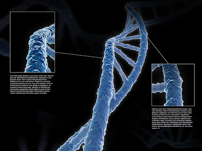
Regardless of the object or environment you’re constructing, you’ll most likely need some sort plan to ensure that all bits and pieces ends up at their right location. So does nature. DNA constitutes the gene pool of all known living organisms, and serves as a blueprint to life itself. While today’s biology lesson could easily turn into a fascinating discussion about Deoxyribonucleic acid (DNA), the theories of evolution and why not the essence of our existence, I’m afraid it will probably be the shortest class you have ever attended. As the word itself is almost to complicated to even pronounce, I want even attempt to provide you with any deeper explanation on the subject.

Browsing trough some medical image libraries for references, we’ll se that there’s a couple of different popular styles to illustrate DNA. Choosing which style (and colors too, for that matter) to use isn’t merely an artistic choice though. Depending whether the purpose of the illustration is to provide any kind of truthful biological information or if it’s simply a really nice image, will either limit or broaden your options. Well, since we’re in a somewhat unscientific mood today, we’ll try to approach the shading in broader more general way. So our texture nodes of choice and their values are by no means any exact science, and should rather be used as guidelines, hopefully giving you the insight enabling you to easily modify the material to better suit your specific needs.

Even as I in general tend to prefer the control gained when working with painted textures, there are many situations where procedural textures just come really handy, and this is surely one of those. As conventional images are resolution dependent you can only scale them so much before they start falling apart, while the procedurals don’t have this drawback. This can become a crucial issue when you’re setting up bump and displacement maps, as the deformation of the surface relies on the color values retrieved from the texture. As you zoom in on the object, at a certain point artifacts will start showing in the image (due to a to low resolution). These miscalculations will be carried on to the displacement of the surface, creating unwanted effects. Another thing we’ll need to be aware of is how the bump and displacement mapping is handled by Softimage. By default, all shades brighter that pure black will push the geometry outwards from its original position, where completely black areas will remain unaffected. Well, this isn’t entirely what we want, so we’ll need to make some adjustments. We only want the areas that are brighter than 50% gray to push the geometry outwards, whereas those with a value less than gray to be pulled inwards. Furthermore, we want a mixture of several textures to drive the displacements, creating irregularities with different shapes and sizes. While these wishes are rather straightforward to achieve in the render tree, the solutions might not be completely obvious. Keep in mind that in order for the displacement mapping to function properly, you need to set the appropriate parameters in the Geometry Approximation property page of the object. While this was already taken care of in this Q&A, these settings will have an impact on the quality of your displacement as well as on the render time, so it’s something that you definitely should try tweaking on your own.

To attain a nice variation of the DNA’s color, we’ll make use of a couple of different techniques. First we’ll blend the main diffuse color depending on the surfaces angle in relation to the lights in the scene. On top of that we’ll give the string a colored volume, before finishing it of by making parts of it appear slightly self-illuminated. While some of the effect might be subtle on their own, they will make a difference in the final image. Notice that the geometry’s overall shading is primary obtained from the mixing of nodes in the Render Tree, rather than requiring any complicated setup of different light sources. As the material we’re aiming for essentially is about combining those different nodes, the render tree can quickly become a bit cluttered in the step-by-step procedure, so please bear with me. If you do find yourself lost somewhere along the line, you can open the scene DNA_final.scn from the cover CD and examine the finalized render tree till you feel confident recreating it on your own.

The project files used in this tutorial can be found at:
http://www.Redi-Vivus.com/Caffeineabuse/DNA_Shader.zip

DNA Step by step
While DNA might be the blueprint of life, these steps are the blueprints for the DNA itself.
Open the DNA scene from the cover CD-ROM. As you can see there are two deformers applied to DNA string. First we have the Twist deformer that obviously twists the string around its own axis. The second deformer is a path deformer, which enables you to alter the overall shape of the string by moving the points on the curve. Adjust the parameters till you’re happy with appearance of the string and set an appealing camera angle.
Apply a Lambert shader to the DNA and set the Ambient to pure black. Open up a Render Tree and get an Incidence (Nodes>Illumination) and a Mix 2 Colors (Nodes>Mixers). Connect the later to the diffuse input of the Lambert node. Set the Base color to a medium dark blue (R:0,207 G:0,256 B:0,7) and the Mix Layer to a pink shade (R:0,994 G:0,256 B:0,7). Connect the Incidence node to the weight input and open its PPG. Change the Mode to Surface/Lights. Set the Bias to about 0,15, the Gain to 0,95 and check the Invert box.

Next we’ll give string a sense of volume, so Lambert PPG set the Transparency to a light gray (RGB:0,7). Get the following nodes: State>Scalar state, Math>Change Range, Math>Scalar Exponent and another Mix 2 Colors. Connect the Scalar state to the input of the Change Range node. In the PPG set the New Range:Start to 0, the End to 0,5 and connect this node to the Scalar Exponent. Change the operation to Logarithm, lower the Factor to 0,01 and connect this node to the weight input of the Mix node.
In the Mix PPG, set the Base color to a dark blue (R:0,055 G:0,207 B:0,466), the Mix layer to pure white and connect the node to the Volume input of the Material Node. Now we’re starting to get some interesting results, though the surface of the DNA is way to uniform and dull. So to fix this we’ll apply two different displacement maps, one for the broad deformation and a second to add a bit of more details. For this we’ll need the following nodes:


Nodes>Texture>Rock, Mixers>Mix 2 Colors, Image Processing>Color Correction and finally a Math>Change Range node. Open the PPG of the Rock node. Set the Grain Size to 0,75, the Diffusion to 0,1. Under the Advanced tab, change the UV maximum remap to 1. Connect it to the Base Color of the mixer node. Now, create a copy of the Rock node and invert color 1 and 2. Set the Grain Size to 0,2, the Diffusion to 0,1 and connect it to the Mix node as color 1. Connect the Mix node to input of the Color correction and lower the contrast to about 0,15.
Connect the color correction to the input of the Change range node. Set the New Range:Start to –0,5, the End to 0,5 before connecting the branch to the Displacement input of the Material node. Go back to the Rock nodes and apply a Spatial texture projection. As a final touch, open the Lambert PPG. Under Indirect Illumination, set the Incandescence to a light blue color. Click on the Connection icon next to the Intensity slider and choose Incidence. Check the Invert box in the PPG and your DNA string is completed…

A couple of additional tips

There’s really no excuse for not upholding the bigger picture, so make sure you’re not lost in the microscopic world of DNA with the help of these tips.

Tip #01

Trying out different settings in the various nodes can become a bit tedious once the tree is getting more complex. As the complexity of the tree increases, so does the render time required to preview your alterations. To speed up your workflow, only preview the nodes your working on. If you’re for example is trying to sort out your preferred values of the Rock node, there’s really no need to calculate the displacement, volume and color of the object. Disconnect all the nodes from the Material and plug in the Rock branch directly to the Surface input. This will give you shade your object with a correct representation of your settings, but at a fraction of the render time. In the early versions of XSI you could preview the branch you currently where working on by the press of a button. Though the hotkey was removed due to stability issues, you can still reactivate it in the Keyboard Mapping menu inside of XSI. While it’s a great time saver, please note that it might not be completely safe to use (hence the removal in the first place), so handle with care.

Tip #02
As you start adding nodes to the render tree, it doesn’t take long before they start piling up and finding the right node is almost wishful thinking. To keep track of your nodes it’s a very good idea to acquire the habit of naming them, and preferable with a naming convention that make some sort of sense. Not only will you regain the overall control and readability, but if you ever open an old material you might actually understand the purpose of each node in the tree.

Tip #03

While we made use of the Rock node for the displacement of the surface in walkthrough (mainly because it’s easy and straightforward to set up) you can get a wide range of differently shaped patterns by using any combination of the other procedural nodes. However, you’re not limited to purely make use of the procedural, as you can mix and match them with standard textures/images as well.

Read the full post>>

2.5D Shading

The Gradient node, warm and vivid colors and a generous use of subdivision - the three key ingredients for a truly snugly and cozy scene

It’s kind of funny to see that the world of 3D hasn’t been spared from trends and the desire to dress in whatever that happens to be the latest fashion at the time. Though we might not have an official spring collection coming out each year nor the fancy vernissage held by the design houses from the cloth industry, we still have vogue in some manner. As they should, the trends do have shifted quite a bit during the past decade. Though I still have occasional nightmares every now and then from the time when people for absolutely no obvious reason persisted on putting lens flares on every single image they created, I must say that today’s obligatory flock of birds aren’t by far that painful as they still leave room for some peace of mind (and the ability to actually se other parts of the image).

The trends don’t end there though. It doesn’t seem that long ago most people where crying for photo-realism in their renderer, which at that time was so much harder to achieve than it is today with the more mature soft- and hardware available. Now when realism is more or less within the grasp of everyone it’s nice to see people talking a step backwards, crying for something completely different. A vogue that’s been popular for some time now, is non photorealistic rendering (NPR) and alike. The ability to create and animate everything in 3D and render it in whatever style needed is not only favorable artistically but also a huge timesaver in comparison to traditional hand drawn animation.

Though you might only need two and a half dimensions to give your image just the right touch, you still have to create all three of them. It’s valuable to think about how you want your final image to look before you start modeling. It might sound kind of obvious that the way you object will be perceived is not only due to the shader or color you are using but also the character of the shape (this is especially true if you are to use toon shading). If we for example where to use our material in a technical illustration or animation with mainly flat areas and lots of small details it might not only look out of place but could actually fail to produce the desired look. Since we want to add a cartoon feeling to the set, it’s important that our geometry express this as well. In the cartoon world it seems to be very troublesome to get hold of completely flat or straight objects. Therefore most things found in there have a tendency to be kind of soft or bulgy, even if it would make them erroneous in our world. This is easily accomplished in XSI by a generous use of subdivisions. This ensures that the entire scene is kept as snugly and comfortably as we need it to be.

There’s no reason why we should end it there. Being so close to taking coziness to a whole new level we might as well give it shot. When setting up the color scheme for your scene, try to make use of as vivid colors as possible. You don’t have to limit the selection to warm colors exclusively, since coloring part of the image with any shade from the cool half of color wheel will only add to the richness of the scene. With our color scheme all set we just need to come up with a method that will get the shading across the surface just smooth enough to add the half dimension to a flat 2D drawing. Once done with the solution you are about to familiarize yourself with, it will appear as the easiest thing; the only tricky part is probably figuring out that it’s there. The core of our material is in fact nothing more than a Gradient node. It is however important that you use the right gradient node. We’re not going to use the one found under Nodes>Texture in the Render Tree, but the one under Node>Texture Generators. What’s the difference then? Well, the difference related to this scenario is the ability to use an Incidence node to drive the mapping of the gradient. This enables us to control the gradient depending on the surface’s angle to the camera instead of fiddle around with texture projections.

The project files used in this tutorial can be found at:
http://www.Redi-Vivus.com/Caffeineabuse/2_5D_Shading.zip

0.5 dimensions Step by step
What could possibly be better at this time of the year then a model of flower to really get your material to flourish? Most likely nothing, so start by loading the scene called flower, found on this issues cover CD. This scene contains nine spheres of which eight of them have been modified (by using the Proportional Modeling tool) to form the petals. To create the stalk we’ve deformed a cylinder along a curve.
Select all of the petals, press Ctrl + G to group them and apply a Lambert shader to the group. Open the Render Tree and get a Gradient node from the Node>Texture Generators. Connect it to the ambient and diffuse input of the Lambert node. Open the properties of the Gradient node. By default there’s quite a lot of color markers controlling the gradient but we only need two of them so delete the rest.
Select one of the markers, move it all the way to the left side of bar and give it a clear yellow color. Now select the other marker, move all the way to the right and set the color to a vibrant orange. The markers position and color are by now way fixed, so feel free to use your favorite colors instead. Just make sure there’s clear difference between them. Next switch to the input tab and change the Input Type to Scalar input.
Now, get an Incidence node (Nodes>Illumination), set the Bias to 0,15, the Gain to 0,75 and connect it to the input on the Gradient node. If you draw a render region you can see how the flower is being shaded by the gradient. To make the flower even more vibrant connect the output of the Gradient to the Incandescence of the Lambert node. Under the Indirect Illumination on the Lambert node set the Incandescence Intensity to about 0,2.
Open your Cameras Property Editor, switch to the Lens Shaders tab and apply a Toon Ink Lens shader. Press the Inspect button to bring up its properties. The flower now has an ink line applied to it, but with a constant thickness along all the objects it might be a bit lifeless. So, under Taper tab set the Anisotropy Amount to 1. This will shift the thickness depending on its angel to the camera.
Let’s move on to the next tab, labeled Variation. Set the Spread Amount 0,6 Under Variation change the Min to 0,5. This will add even further variations to the ink, making it appear more natural. Increase the Frequency sliders for additional variations. Leave the rest as it is or preferable, continue trying out different parameters and setting on your own until your pleased with the result.


A Couple of additional tips
Half dimensions, rendering settings and fuzziness, all nicely wrapped up with these expert tips.


Tip # 01
Still feel that something is missing? Well, a subtle bumpmap will break up the uniformity of the color, giving it an almost fuzzy look, which might be just what you need for that final touch. Add a fractal node (or alike) or use the image found in the Pictures folder on the cover CD.

Tip # 02
A little too much depth in your image? Depending on what style you are trying to give your rendering you might actually benefit (or make do) without the Lambert shader in your material. By connecting the output of the Gradient node directly to the Surface input of your Material you will reduce some of the depth in your image, giving it more of 2 dimensional feeling. Another plus from getting rid of the Lambert node is that your materials aren’t depending on the lights for their shading anymore, and without the need of lights the rendering time is bound to go down.

Tip # 03
Whenever working with the toon ink lens shader one must unfortunately be prepared to take a hit on the rendering time. To optimize your rendering and avoiding the risk of flickering when your animation is played back, you should tweak the settings in the Render Property Editor as well as those found under the Sampling tab in the Toon Ink Lens Property Editor. Though the last of these is supposed to be enough to control the sampling of the ink, one should fiddle with both of them to find the best settings for a particular scene. The thicker and complex your ink is the more sample will be needed to maintain the quality. As always you should keep these settings rather low to speed up the previews, then increasing them when it’s time for the final render.

Tip # 04
Another way to approach the 2.5D type of rendering would be to combine two or more versions of the same scene, which are rendered with different materials. To withhold simplicity for controlling your entire scene you set up the materials within the same scene by using different pass’s and partitions. Use a Constant or Toon shader (or why not try the material created above) as the base for the effect. Create another pass, but use FG/GI to illuminate the scene. Bringing the rendered versions of the passes into the FX Tree and blending them together (either with or without additional filters) can produce some truly interesting images.

Read the full post>>

Lattice Rigging

I guess most of us just think about paper bags as a very practical way to carry our merchandises home from the supermarket, or to stockpile all kind of weird bits and pieces in the closet, though you know you have absolutely no intention of ever using them again so you really ought to toss it right away; but as one of our readers found out, there obviously are other fields of application for them as well.

The paper bag is in fact a relatively old innovation and was mentioned in Europe as early as during the seventeenth century. Tough they where folded and glued by hand during that time they still have the same characteristics - a void, surrounded on five sides by a thin piece of paper.

Most paper bags are constructed in the same manner, a tube of paper, which is folded together at the bottom. Part from obvious differences such as size and color, one of the few things that differ an everyday bag from a more luxurious model is usually the added coating/finishing and quality of the paper and the handles. The ones you get at an expensive design store for example usually have nice shiny surface and handles that are made by stings of fabric or plastic instead of the same unexciting paper as the rest of the bag.

So how do we animate an object that hasn’t got any part that even comes close to resembling a leg, face or limb for that matter? Well, by taking a second look at the bag we might find out that the above assumption isn’t necessarily true. Even though the bag is monotonously shaped, it at least has four corners and in the middle of those corners there obviously is a center. Take these and add a bit of imagination and we all of a sudden have two feet, two shoulders and a hip. Quite good ingredients for a character animation in other words. Despite our newly invented limbs, the shape of our object would still make it somewhat inconvenient to be setup and animated with bones, so we could benefit from another solution.

We’ll approach the problem with a basic, but for this task, very suitable method. In fact the entire deformation of the object will be controlled by a single lattice with the resolution (or subdivision) set to create areas that corresponds with the “body parts” we are about to animate. This enables us to control the geometry with very few points while still being able to create complicated poses.
Since it is not possible to animate the actual points directly with the standard SRT tools in XSI (without using Shape Keys) we need to add one more thing to facilitate the animation process. By constraining the points to different Null or Implicit objects and animate these instead we’ll make it easier to select and transform any of the parts. Implicit objects are like Nulls with another shape, which can be an advantage when trying to distinguish them in a cluttered scene for example.

Since we quite seldom, to say the least, get the chance to see paper bags walking around out of their free will we need to find something else to base our movement on. Conveniently the movement of a human will translate very well, but since it still is a paper bag we’ll loosening it up to give it a slightly cartoonish walk. The walk can say a great deal about a person’s character, such as gender, age, physique, frame of mind, etc. Given that no two persons therefore walk identical the appearance or design of a walk is never-ending. The idea on the next page is to show you the basic of setting up and animate the paper bag. To keep things simple it can be helpful animating one or two parts at the time. You can for example start with the feet. Once satisfied with the way they move, you can start working on the other parts. The bag’s true personality is something you will give it. As you start playing around with the bag you will probably find different posses and timing that better suits your needs, but you have gained the understanding how to realize them.

If we successfully manage to tie all of the above together, we’ll end up with a nice and easily controlled animation of our newly found friend, so enjoy.

The project files used in this tutorial can be found at:
http://www.Redi-Vivus.com/Caffeineabuse/Lattice_Rigging.zip

Paper Bag Step by step - Get your paper bag up and running with these six steps
If you haven’t got a model standing by, load the scene called paper_bag.scn from the magazine cover CD. The geometry of the paper bag is quite uncomplicated and was basically constructed with a Cube where the top polygon has been deleted. Edges were then added to create the creases before giving it its overall shape. Since the paper is extremely thin, there’s really no point adding twice the amount of polygons to create the inside.
Select the paper bag and create a Lattice. By having the object you want to deform selected the Lattice will automatically be created with the right dimensions and at the right position. Set the X Subdivision to 3, the Y to 3 and the Z to 1. With the Interpolation set to Linear, the deformation will be a bit to pointed so change both the X,Y and Z to Curve.
In this environment it can be difficult to spot a Null, so start by creating an Implicit Cube instead and name it Hip. Set the length high enough for the borders of the Cube to reach outside the bag and position it in the middle of the four center points of the Lattice. Create four new Implicit Cubes and position one at each corner. Name them lt_foot, rt_foot, lt_shoulder and rt_shoulder.
Next we need to constrain the different areas of the Lattice to the respective Cube. Start by selecting the four center points on the Lattice and choose Deform>Cluster Center and pick the Hip cube. Move on by selecting the three points in the lower right corner, apply another Cluster Center and pick the corresponding cube. Repeating the previous step for the remaining corners. You can now hide the Lattice to get a clearer view.
To create a simple step we need at least four different poses. Let’s start by creating the position where both feet touch the ground. Change the selection filter to Implicit to make the selection easier. Move lt_foot and rt_sholder forward and rt_foot and lt_sholder backwards. Set a keyframe. Go to frame 9 and move the hip and rt_foot slightly forward and upwards. Move rt_shoulder forward as well and set a new key for all Implicits.

At frame 18 move the lt_foot forward and lower it so it touches the ground again. Move lt_shoulder and the hip forward, but lower the hip as well. Set a key. At frame 27 move the hip and lt_foot forward and up and both shoulders forward. At frame 36 move all Implicits forward, except lt_foot. Lower the hip and rt_foot. Play the animation back and forth. Try experimenting by adding rotation to the objects and animating the shoulder going up and down as well. Open the Animation Editor and fine-tune your curves…





A couple of additional tips

Tip # 01
Although the setup in the step by step guide gives you a neat and swift way to animate your bag, there are times where your animation might call for a specific pose, expression or the need to control the sides individually. This can be very difficult or just isn’t achievable with the current setup. To bypass this, increase the subdivisions on the lattice to allow more areas to be controlled separately. By constraining the new areas to new Null or Implicit objects and putting these in hierarchies with the old Nulls as the parents, you can maintain the simplicity of the original setup but with the extended control. The above technique can then be used either in conjunction with Shape Keys and the Animation Mixer or entirely replaced with by it.

Tip # 02
If you are using Nulls instead of implicit objects as the deforming object for the Cluster Centers you can save a mouse click or two. By selecting the desired points and choosing Create Cluster with Center under the Edit menu, a Null will automatically be created and the points constrained to it.

Tip # 03
Often when working on animations you should try to keep everything as smooth as possible, but there are occasions when you don’t want that, and if you are aiming for grater realism this is one of those. Try playing around with a real paper bag for yourself and you will see that it in fact has no intention what so ever of deforming smoothly. Instead you tend to get lots of somewhat flat areas and creases whenever you fold the paper. So by not overdoing the tessellation or subdivision of the object, but rather keeping the surface at a fairly low or medium polygon count can actually add to the realism of your animation.

Tip # 04
You can use different textures and materials for the inner and outer surface of your paper bag by connect the materials to the respective input of the Front-Back node. This node can be found in the Render Tree under Nodes>Switch.

Read the full post>>