Create dimples when particles collide with the surface

Just a few years ago (or versions of Softimage if you will) this type of effect would require a fair amount of time and patience and certainly wasn’t something you would whisk together in three little steps. By using ICE there’s actually very little information you need to extract from the scene in order to create the dimples. You obviously need to find the whereabouts of the particles and the points on the geometry you want to dent but that’s about it.

The project files used in this tutorial can be found at:http://dl.dropbox.com/u/3834689/CaffeineAbuse/Dent_by_particle.zip

Extract particle’s positions
Open the scene Dent_Geometry_by_Particles.scn from this issues CD. Select the grid and press [Alt] + [9] to open an ICE Tree. From the Create menu choose Simulated ICE Tree. Press [8] to open an Explorer and drag and drop the PointCloud into the ICE Tree. Get a Get Closest Location on Geometry node and a Get Data node. Connect the [PointCloud]:Value —> Geometry1:[Get Closest Location on Geometry]. Open the Get Closest Location on Geometry PPG and set the Cutoff Distance to 0.5. Connect [Get Closest Location on Geometry]:Location to the Source:[Get Data]. Open the Get Data PPG and type PointPosition as reference. The next step is to extract the position for each point on the grid and calculate the distance between the grids points’ position and the particles.
Control the magnitude
Get a Get Data node and type self.PointPosition as reference. Get a Get Distance Between and a Rescale node. Connect [Get self.PointPosition]: Value —> First:[Get Distance Between] and [Get PointPosition]:Value —> Second:[Get Distance Between]. Connect [Get Distance Between]: Result—> Value:[Rescale] and open its PPG. The Rescale node will be used to control the magnitude of the dents. A high value will make the effect of the collision more severe whereas a low value will make it more subtle. The output of the Get Distance Between node is a positive value which means you’ll need to invert it to push the geometry inward rather than outwards. Change the Target End value to -0.35.
Deforming the geometry
Get a Get Data node and set the reference to self.PointNormal Get a Multiply by Scalar node. Connect [Get self.PointNormal]:Value —> Value:[Multiply by Scalar] and [Rescale]:Result—> Factor:[Multiply by Scalar]. This will determine the in which direction the points will be pushed. Get another Get Data node and set the reference to self.PointPosition. Get an Add node and connect the Value output of the [Get self.PointPosition] to the Value1 input of the [Add] and the Result [Multiply by Scalar] to the Value2. Get a Set Data node and set the reference to self.PointPosition. Connect [Add]:Result —> self.PointPosition:[Set Data node] and [Set Data]:Execute —> Port1:[ICE Tree]

Read the full post>>

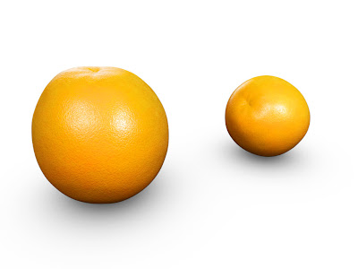
Procedural orange skin

There’s a vast variety of oranges and citrus fruits, each with their distinguished color, shape and texture. But they can all be created using the same basic set of nodes.

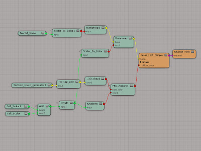
Open the scene orange.scn, select the Orange and press [7] to open a Render Tree. From the Nodes > Texture menu get a Cell Scalar node and open its PPG. Many of the changes made to the nodes are subtle and may be hard to see solely relying on the shaderball. To get a better view of how the values affect the output you can temporary connect the current node directly to the Surface input of material node and draw a render region in the viewport. Change the Fill Color to 0 (zero) and the Border color to 0.8 to create the first set of dark dimples. Increase the Minimum Contrast to 0.35 and the Maximum to 0.65 to give it a more circular shape and lower the Bias to 0.1 Switch to the Texture Support tab. Change the Pre-Scale to Small Noise and set the Scale to 1.5

Get a new Cell Scalar node and set the Fill color to 0 and the Border color to 0.8. Change the Min to 0.3, the Max to 0.8 and the Bias to 0.1. Switch to the Texture Support tab. Set the Pre-Scaling to Small Noise and the Scale to 0.75. From the Nodes > Math menu, get a Scalar Basic node (leave the default math Operation at Add) and connect the first Cell_Scalar node to input1 and the second to input2. Get another Scalar Basic node and connect the first scalar math node to input1 and open the PPG. Set the Input 2 value to 2 and change the Operation to Divide. By first adding the two cell’s value and then dividing them you’ve effectively calculated the average of the two.

From the Nodes > Mixers menu get a Gradient node. Connect the output of the Divide node to input of the Gradient node and open the PPG. Click the Black/White Preset button to remove all but two markers. Change the color of black marker to a medium orange color, such as R:0.07, G:0.47, B:0.85. Set the color of the white marker to a slightly brighter more vivid orange, R:1, G:0.6, B:0.

Get a Cloud node (Nodes > Texture Generators) and a Texture Space Generators node (Nodes > Texture Space Generators). Open the Texture Space Generator PPG and select the Spatial projection. Close the PPG and connect it to the coord input of the 3D_Cloud and open the Cloud PPG. Increase the Level Decay to 0.85 and the Frequency Multiplier to 3. Set the Color 1 to a vivid orange R:0.9, G:0.61, B:0 and Color 2 to a somewhat darker R:0.92, G:0.45, B:0.1. Get a Mix 2 Colors node (Nodes > Mixers), open the PPG and set the Weight to RGBA: 0.35. Connect the 3D_cloud to the base_color input and the Gradient to the color1 input.
Connect the Mix_2colors node to the Ambient and Diffuse input of the Blinn node.

Get a Fractal Scalar node (Nodes > Texture) and open the PPG and set the Contrast Clamp Minimum to 0 and the Maximum to 1. Switch to the Noise tab and increase the Recursion Level to 5. Set the Scaledown to 3.3 and the Gain/Smooth to 1.5 and close the PPG. Get a Bumpmap node (Nodes > Bump) and connect the Fractal_Scalar node to its input. Open the PPG and set the Bump Scale to 0.05 and the Sample Spacing to 0.005. Get another Bumpmap node and set the Scale to 0.025 and the Sample Spacing to 0.015. Connect the Divide node to the input of connect the previous bumpmap node to its bump input. Connect the Bumpmap node to the Bump Map input of the Material node.

The project files used in this tutorial can be found at:http://dl.dropbox.com/u/3834689/CaffeineAbuse/OrangeSkin.zip
Quick tip
While you have the dimples in place you do need a touch of sub surface scattering to sell your orange. Get a Fast Sub-Surface Scattering node (in the Illumination category) and connect the Gradient node to the Diffuce_Color input. Connect the SSS node to the Material input of the Material node.

Read the full post>>

Using individual textures in shared materials

The texture maps, which hold both the actual texture and the UV Coordinates, are assigned directly to the object.

The reason you apply the same material on multiple objects in the first place is usually because you want them to be exactly the same. That’s pretty much the definition of sharing the very same material. With that being said, let’s discuss how you can setup a shared material but still being able to control parts of it on a per object basis. While this answer confines to using an individual texture, there’s nothing stopping you from adding additional individuality. But then again, if you really want completely different appearance for each and every object you’re probably better of using separate materials in the first place.

Start by opening the scene tubes.scn from this issues DVD. Select the first tube, tube_No1, and from the Get > Material menu choose Blinn. Select the other two tubes and from the Get > Material menu choose Assign Material and pick the first tube to assign the same material. Select the first tube again and from the From the Get > Property > Texture Map menu choose Texture Map. In the Clip section of the Texture Map PPG, click the New button and select New From File… from the menu. Brows to the project folder on the DVD, select the tube_No1.pic image and click OK. In the UV Property section, click the drop down list and select the Tube_UV. Close the PPG. Texture Maps are commonly used to control specific parameters in a scene, such as hair color, particle emission or restricting the areas affected by deformers, using an image. And as such they’re generally not used to actually texture an object. The main difference between the ‘traditional way’ of using an image node in the Render Tree and using the texture map is that the texture map property sits on the geometry/object rather than being part of the material. Repeat the same procedure for tube_No2 and tube_No3 but choose their respective image.

Select any of the tubes and press [7] to open a Render Tree. From the Nodes > Map Lookups menu choose Color. The color map lookup node enables you to extract different types of data from the object, such as a texture map, and use it as a color value in the Render Tree. In the Map_lookup_color PPG, click the Map dropdown list and choose Texture_Map. The texture map lookup of the material is shared between all the objects but since their actual texture maps are unique, they will get assigned an individual texture. Connect the Map_lookup_color node to the Diffuse and Ambient input of the Blinn node.

The project files used in this tutorial can be found at:http://dl.dropbox.com/u/3834689/CaffeineAbuse/Individual_Textures_Shared_Materials.zip

While the texture maps are commonly used to control attributes of an operator rather than using it as an actual texture, there is no reason it can’t be used as such.

Quick tip
An object isn’t limited to using a single texture map, so for additional images such as bumpmaps, simply add a second texture map with respective images and a Color Lookup to use it in the Render Tree.

Read the full post>>

How to offset point position in ICE

In order to offset the particles along their individual axis’s you need to determine their current position and in witch direction they’re oriented.

Start a fresh scene and from the Get > Primitive > Polygon Mesh menu choose icosahedron (any dummy object will do) and set the Geodesic Frequency to 4 to make it a bit smoother. With the icosahedron still selected, press [4] to switch to the Simulate toolbar and from the ICE > Create menu choose Emit Particles from Selection. With the pointcloud selected, press [Alt]+[9] to open an ICE Tree.

Open the Emit from Surface PPG and change the Rate type from Number of Particle per Second to Total Number of Particles and Size to 0.5 or so. By default, the shapes of the points are set to (which may not be totally unexpected) just points. While this is sufficient to determine their position, there’s no way to tell their size or in which direction they’re oriented. So for clarity, change the Shape to Cone. In the Orientation section of the PPG, check the Align to Surface Normal checkbox.

In order to offset you need to extract their current position, which direction they’re oriented and then add the offset along their respective axis. For this to happen, you’ll need to add a few nodes. Get a Get Closest Location on Geometry node, a Multiply by Scalar node, an Add node, a Get Point Position node and finally a set Point Position node.

Start by connecting the Get icosahedron node to the Geometry1 input of the Closest Location on Geometry node. There’s a lot of information that can be extracted from this node, but the one you’re currently interested in is the normal or direction. So connect the Normal output to the Value input of the Multiply by Scalar node and the Multiply by Scalar node to the Value2 input of the Add node. The add node will obviously add a value but you first need to too tell it what it should be added to, which is the original position of each point. So connect the Get Point Position to the Value1 of the Add node. While the ICE Tree is just about finished it will not have any effect on the actual could just yet, as you haven’t told it what to do with the information. Connect the Add node to the Position input of the Set Point Position node and connect the Point Position node to the Port2 Input of the ICE Tree node. The node controlling the actual offset is the Factor value in the Multiply by Scalar node. While you can control it directly in its PPG, it will be far easier to “read” your tree if you use a separate node. Get a Scalar node and connect it to the Factor input of the Multiply by Scalar node. Open the Scalar PPG and set your desired offset.

The project files used in this tutorial can be found at:
http://www.redi-vivus.com/Caffeineabuse/Offset_PointPosition.zip

If your different sizes particles and want compensate for it, you can use a second Add node and add the particle size to the scalar value before connecting it to the Factor input.

Quick tip
Your ICE Tree currently lives in the Simulation Stack which means your offset will be applied every frame. To avoid this you can move the ICE Tree to any of the other stacks, such as the Animation. Press the right arrow in the ICE Tree menu to display the Explorer and drag and drop the ICETree operator to any of the stacks below the Simulation.

Read the full post>>

Stretchy bones in ICE

If the distance between the root and the effector is greater that the sum of the length of the bones the chain should stretch.

Open the scene Stretchy_Bones from this issues DVD. Select the Stretchy_Bones null object and press [Alt] + [9] to open an ICE Tree. From the Create menu choose ICE Tree to create an empty ICE Tree. The idea of stretchy bones or limb stretching is quite simple. If the distance between the root and the effector is greater than the sum of the bones, the bones should stretch. But if the distance is less, the bones should stay unaffected at their default length.

Get a Get Data node and double-click on it to open its PPG. Click the Explorer button and expand the tree root > Kinematics > Global Transform and select the Pos. Get a second Get Data node and type eff.kine.global.pos in the Get Data textbox to get the position for the effector as well. The next step is to calculate the distance between the two objects, so get a Get Distance Between node. Connect the root.kine.global.pos node to the First input of the Get Distance Between node and the eff.kine.global.pos node to the Second input.

Get a Scalar node, open its PPG and enter 4 as the Value. This will set the default length of the First_Bone. Get a second Scalar node and set its value to 3. This will be the default length of the Second_Bone. Get an Add node and connect the first Scalar node to its Value1 input and the second Scalar node to its Value2 input.

Get a Greater Than (>) node, an If node and two Divide by Scalar nodes. Connect the Get Distance Between node to the First input of the Greater Than node and the Add node to the Second input. Connect the Greater Than node to the Condition input of the If node.

To set the new length for each bone you must first determine the ratio of the individual bone’s length and the distance of the root and effector. Connect the Add node to the Value input of the first Divide by Scalar nodes and the Scalar node (with the value 4) to the Divide By input. Then connect the Divide by Scalar node to the Divide By input of the second Divide by Scalar node. Connect the Get Distance Between node to the Value input. Connect the Divide by Scalar node to the If True input of the If node. Connect the Scalar node (with the value 4) to the If False input.

Get a Set Data node and connect the If node to the Value input and open its PPG. Click the Explorer button and expand the Root > Bone > Chain Bone and click the Length. Connect the Set Data node to the Port1 input of the ICE Tree.

To set the length of the Second_Bone repeat the procedure, but use the second Scalar node (with the value 3). Please use the screenshot as reference.

The project files used in this tutorial can be found at:
http://www.redi-vivus.com/Caffeineabuse/Stretchy_Bones.zip

To calculate the new length for each bone you must first determine the ratio of the individual bone’s length and the distance of the root and effector.

Quick tip
The technique used is by no means limited to two bone chains. To use more bones simply add the corresponding Scalar nodes to the Add node, use the Divide by Scalar to get the division factor and connect it to the Set Data node.

Read the full post>>

Changing color of an objects based on its distance to another object

You can use the scalar to vector node to extract the position of an object and make it available in the Render Tree
There are many instances where you want to be able to control an attribute of a shader based on its distance to the camera or another object in the scene. Regardless of the end effect you’re trying to achieve, the procedure of getting there is about the same.

Select any of the spheres (they all share the same material) and press [7] to open a Render Tree. From the Nodes > Conversions menu, get a Scalar to Vector node. This node enables you to enter any XYZ coordinates and by linking their separate values to the corresponding value of the Ctrl_Null, you’ve efficiently extracted the nulls position and made it available in the render tree. Open its PPG and click the Lock icon to pin it to the screen. Select the Ctrl_Null and press [Ctrl] + [K] to open its transform PPG. Drag the animation icon (the green divot) for the X Position (in the transform PPG) and drop it onto the animation icon of the Input X in the Scalar to Vector PPG. Repeat for the Y and Z position.

Rather than extracting the position of the object holding the material, which you can’t do anyway in this scenario since there are multiple objects, you’ll use its intersection point. By comparing the intersection point with the position of the Ctrl_Null you can extract the distance between them. From the Nodes > State menu get a Vector state. Open its PPG and change the State Parameter to Intersection point. From the Nodes > Math menu get a Vector-Scalar node. Open its PPG and change the operation to Distance between V1 and V2. Connect the Scalar to Vector node to the vector_input1 of the Vector_math_scalar node and the Vector state to the vector_input2. Depending on the scale of your scene the distance value can be extremely small or large so you’ll have to change its range to something more useful. From the Nodes > Mixers menu get a Gradient node and a Mix 2 Colors node. Connect the Vector_math_scalar node to the input of the Gradient node and the Gradient node to the Weight input of the Mix_2colors node. Connect the Mix_2colors node to the ambient and diffuse input of the Blinn node.

Open the Gradient PPG and switch to the Input tab. In the Active Range section, change the Maximum to 20. Switch back to the RGBA Gradient tab and click the Black/White preset. The minimum and Maximum values in the Active Range controls at which distance the Ctrl_Null start effecting the material and the gradient controls the falloff of the effect. So for a sharper falloff, simply move the markers closer together.

The project files used in this tutorial can be found at:
http://www.redi-vivus.com/Caffeineabuse/Modify_Color_By_Distance.zip

You can then compare the position of the object with the intersection point on surface to extract the distance between them.

Quick tip
To further enhance the effects falloff you can add a third marker in the middle of the gradient and connect a greyscale texture, such as a fractal, to it. This way you can breakup the regularity of the transition from black to white.

Read the full post>>

Assigning different task based on condition

Select the particle_emitter and Simulate > ICE > Create menu choose Emit Particles from Selection… With the PointCloud still selected, press [Alt] + [9] to open an ICE Tree. Before you can assign any goal or paths for the particles you have to choose a criterion to use to separate the particles. In this example you’ll be using three different objects so it makes sense to divide the particles into three groups, one for each goal/curve. As each particle is born it’s also assigned a unique identification or ID. By feeding this ID into a Modulo operation and set the devisor to the same value as the number of groups you want to create, you’ve efficiently created the 3 collections.

Get a Get Point ID, a Modulo and a Set Data node. Connect the Point ID to the Value input of the Modulo node. Double-click on the Modulo node to open its PPG and set the Modulo By to 3. Connect the Result of the Modulo node to the Value input of the Set Data node. Open the Set Data node’s PPG and in the reference textbox enter self.Goal_ID. This creates a custom variable where each particle is assigned the result from the Modulo node (which is one of three numbers 0, 1 or 2). Connect the Execute port of the Set Data node to the Execute on emit1 input of the Emit from Surface node.

Get a Get Data node and a Select Case node. Open the Set Data PPG and enter self.Goal_ID in the text box and close the PPG. Connect the Value port of the Get Data node to the Condition input of the Select Case node and the Select Case node to the Port2 input of the ICETree node.

Press [8] to open an Explorer. Select the goal object and the two curves and drag and drop them into the ICE Tree. Get a Move Towards Goal node and connect it to the Case0 input of the Select Case node. Connect the Value port of the Goal_No1 node to the Geometry1 input of the Move Towards Goal node. Get two Flow Along Curve node and connect the each Curve node to the Curve1 input of their respective Flow Along Curve node. Connect the execute port of the first Flow along Curve node to the New (Case0)… input of the Select Case node and the second Flow along Curve node to the New (Case1)… input.

The project files used in this tutorial can be found at:
http://www.redi-vivus.com/Caffeineabuse/Multiple_Goals.zip
Image 01
Rather than staking numerous If or Filter nodes, the Select Case node can be used as an efficient way to execute different tasks based on conditions
Image 02
Becoming acquaintance with the Modulo operator will save you a lot of time whenever you need to separate particles into different group or collections.

Quick tip
If you’re using multiple goal objects, replace the Move Toward Goal node with a Set Particle Goal node. On the ICETree node, right click on the Port3 and from the menu choose Insert Port Before to insert a new port. Get a Move Towards Goal node and connect it to the Port3 input of the ICETree node. This way you can control all the particles within a single node even though they have separate goals.

Read the full post>>