Assigning different task based on condition

Select the particle_emitter and Simulate > ICE > Create menu choose Emit Particles from Selection… With the PointCloud still selected, press [Alt] + [9] to open an ICE Tree. Before you can assign any goal or paths for the particles you have to choose a criterion to use to separate the particles. In this example you’ll be using three different objects so it makes sense to divide the particles into three groups, one for each goal/curve. As each particle is born it’s also assigned a unique identification or ID. By feeding this ID into a Modulo operation and set the devisor to the same value as the number of groups you want to create, you’ve efficiently created the 3 collections.

Get a Get Point ID, a Modulo and a Set Data node. Connect the Point ID to the Value input of the Modulo node. Double-click on the Modulo node to open its PPG and set the Modulo By to 3. Connect the Result of the Modulo node to the Value input of the Set Data node. Open the Set Data node’s PPG and in the reference textbox enter self.Goal_ID. This creates a custom variable where each particle is assigned the result from the Modulo node (which is one of three numbers 0, 1 or 2). Connect the Execute port of the Set Data node to the Execute on emit1 input of the Emit from Surface node.

Get a Get Data node and a Select Case node. Open the Set Data PPG and enter self.Goal_ID in the text box and close the PPG. Connect the Value port of the Get Data node to the Condition input of the Select Case node and the Select Case node to the Port2 input of the ICETree node.

Press [8] to open an Explorer. Select the goal object and the two curves and drag and drop them into the ICE Tree. Get a Move Towards Goal node and connect it to the Case0 input of the Select Case node. Connect the Value port of the Goal_No1 node to the Geometry1 input of the Move Towards Goal node. Get two Flow Along Curve node and connect the each Curve node to the Curve1 input of their respective Flow Along Curve node. Connect the execute port of the first Flow along Curve node to the New (Case0)… input of the Select Case node and the second Flow along Curve node to the New (Case1)… input.

The project files used in this tutorial can be found at:
http://www.redi-vivus.com/Caffeineabuse/Multiple_Goals.zip
Image 01
Rather than staking numerous If or Filter nodes, the Select Case node can be used as an efficient way to execute different tasks based on conditions
Image 02
Becoming acquaintance with the Modulo operator will save you a lot of time whenever you need to separate particles into different group or collections.

Quick tip
If you’re using multiple goal objects, replace the Move Toward Goal node with a Set Particle Goal node. On the ICETree node, right click on the Port3 and from the menu choose Insert Port Before to insert a new port. Get a Move Towards Goal node and connect it to the Port3 input of the ICETree node. This way you can control all the particles within a single node even though they have separate goals.

Read the full post>>

Painting weights in ICE

While the weights in the weight map will be controlled from within the ICE Tree, you have to create the actual weight map manually. Select the Grid object and from the Get > Property menu choose Weight Map. Select the Grid object and press [Alt]+[9] to open an ICE Tree and from the Create menu choose Simulated ICE Tree. Press [8] to open an Explorer and drag and drop the Sphere object to your ICE Tree. Continue by getting a Pass Trough node, a Get Point Position node and a Get Closest Location node. The Get Point Position node returns the position of each of the points of the grid which is then used by the Get Closest Location node to determine whether the Sphere touches any of the vertices of the grid object (or is within a specified distance). If the Sphere is within this value the corresponding points’ weight should be set 1. If it’s not, the weight should stay unaffected (the default value is zero). Open its PPG. Check the Enable Cutoff Distance checkbox and set the Cutoff Distance to 0.1 and close the PPG.

Connect the Get Sphere node to the In input of the Pass Trough node, and the Pass Trough node to the Geometry input of the Get Closest Location node. The Pass trough node is purely for assisting the creation of compound (see Quick Tip). Connect the Get Point Position to the Position input Get Closest Location node.

Get a Set Data node and double click on it to open its PPG. The Set Data node can be used to set any predefined value or, as in this case, a custom value. In the Reference text box enter self.AddWeight. This will create a custom property named AddWeight. While you can set the value directly from within the PPG, using a separate node for this will make it easier to ‘read’ the ICE tree just by looking at it. So, get a Scalar node set its Value to 1 and connect it to the self.AddWeight input of the Set Data node. Get a If node and connect the Found output of the Get Closest Location node to the Condition input of the of the If node. Then connect the Set Data node to the If True input of the If node. Get a Execute node and connect it to the Port1 input of the ICETree node. Then connect the If node to the Port1 of the Execute node.

Get a Get Data node and open its PPG. Enter self.AddWeight in the Reference text box. Get a Set Data node, open its PPG and click the explore button. In the Explorer, expand the Grid > Polygon Mesh > Clusters > WeightMapCls > Weight_Map and select the Weights node. In the Reference text box, replace the word Grid with self and close the PPG. Connect the get self.AddWeight node to the self.clsWeightMapCls.Weight_Map.weights input of the Set Data node. Conclude the tree by connection the Set Data node to the New (port1) input of the Execute node.

The project files used in this tutorial can be found at:
http://www.redi-vivus.com/Caffeineabuse/ICE_WeightMaps.zip
Image 01
A weight map essentially enables you to store a weight value for each point of an object (or part of your object if you’re using clusters)...
Image 02
…which can be used to control anything from particle emission, shape animation and deformers to defining custom material properties of on object.

Quick tip
In the ICE Tree, select all but the Get Sphere and ICETree node, and from the Compounds menu choose Create Compound. Your ICE compound can now easily be saved to your library for later use.

Read the full post>>

Expanding the width of the rendered image without distorting the camera perspective

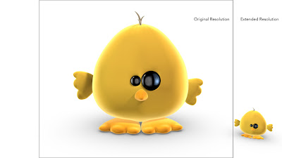
By changing the cameras position and increase the size of the output resolution you’ll obviously be able to widen the shot. Unfortunately you’ll end up with a completely different perspective. By compensating the cameras field of view angle in relation to the added pixels the expanded images will line up exactly with the original image when superimposed. The procedure will work just as well if you need to reduce the size of the image.
Step 01
Determine the scaling factor
For example let’s assume that your original rendered image is 800 pixels wide and you would like to add 200 pixels to each side making it 400 pixels wider in total. To determine the scaling factor simply divide your desired resolution with the original, which in this scenario is 1200 (800+400) by 800 which equals a scaling factor of 1.5.
Step 02
Changing the Film Aperture
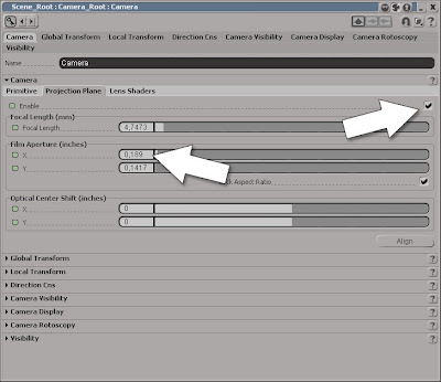
In the Camera viewport, click on the Camera icon menu button and choose Properties from the menu to open the Cameras PPG. Switch to the Projection Plane tab and check the Enable checkbox. Please note that depending on whether you want to increase the width of the image or the width and the height you’ll need to check or uncheck the Lock Aspect Ratio checkbox in the Film Aperture section prior to changing its values.
Step 03
Changing the output resolution
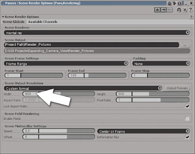
In the Film Aperture X text box enter 1.5* (which is the scaling factor) and press [Enter] to multiply the original value. Close the PPG and press [3] to switch to the Render Toolbar. From the Render > Render menu choose Scene Options… to open the PPG. In the Scene Output Resolution section enter 1.5* in the Width textbox and press [Enter]. Don’t forget to check/uncheck the Lock Aspect Ratio here as well prior to multiplying the values.

Read the full post>>

How to fill a volume using rigid body dynamics in ICE

The rigid body dynamics in ICE does not only compute faster than the traditional RBD in Softimage, it also turns the handling of thousands of delicious coffee beans into a no-brainer.

The standalone or default rigid body dynamics engine is the preferred solution if you’re simulating few or a fixed number of objects and need high precision. If you’re on the other hand are set to take on a large number or are adding new objects to the simulation over time then ICE would most likely be the one to choose. Even as booth engine uses the physX as the dynamics engine, ICE still isn’t the answer to all your upcoming simulation struggles. And the reason for this is quite simple. Kinematics isn’t officially supported within the ICE framework yet (though it can be activated manually) and the actual shape isn’t available as a collision type.

Open the scene fill_bag.scn from this issues DVD. Press [4] to switch to the simulation Toolbar and select the bean_emitter. From the Simulate > ICE > Create menu choose Emit Particles from Selection. With the PointCloud selected, press [Alt]+[9] to open the ICE Tree. Double click on the Emit from Surface node to open it’s PPG. Change the Size to 1 (which translates to 100 percent of the instanced geometry size). Since the actual shape isn’t supported you’ll have to make do with the next best thing, convex hull. The convex hull is an approximation of the objects actual shape and thus is much faster to calculate. The drawback is that it doesn’t take any holes or dents into account, which can become a bit of a problem since you’re trying to fill, that’s right, a hole! The solution to avoid this obvious bottleneck is to break the object into a number of flat objects and use these as the obstacles.

Get an Instance Shape node, open its PPG, click the Explorer button and choose the CoffeeBean object. Close the PPG and connect the node to the Shape input of the Emit from Surface Node. As you’re merely trying to get those rich and tasteful little beans into the paper bag, a simple gravity force will do the trick. Get an Add Forces node and connect it to the Port 2 input of the ICETree. Then get a Gravity Force node and connect it to the Force1 input of the Add Forces node. Since you’ll be using RBD to compute you don’t need the Simulate Particles node so simply delete it. Instead, get a Simulate Rigid Bodies node and connect it to the Port 3 input of the ICETree node. Open the Simulate Rigid Bodies PPG and change the Elasticity to 0 to keep the beans from bouncing straight out from the bag. Press [8] to open an Explorer and drag and drop the Bean_Obstacles group into the ICE Tree. Connect the obstacles node to the Obstacles > Geometry input of the Simulate Rigid Bodies node.

The project files used in this tutorial can be found at:

http://www.redi-vivus.com/Caffeineabuse/Fill_Volume.zip

The obstacles will be used in the simulation even if they’re not visible so you can hide the obstacles group and the bag to get a clearer view of your beans.

Quick tip
While the actual shape isn’t available as an optimized one-click solution, the same end result can be achieved by extracting each individual polygon of your obstacle as a separate object. Make sure you add a bit of depth to objects as this will assist the accuracy of the simulation.

Read the full post>>

Rigging a piston engine

Image 01
For the reason that the relation between the crankshafts rotation and the pistons y position isn’t linear, a standard position constraint won’t cut it.

The concept of a reciprocating engine, commonly referred to as a piston engine, is in fact quite simple. Petrol gets injected into the cylinder and the piston pushes upwards to compress the petrol (fumes). The spark plug sets of a spark which ignites the fumes and causes it to explode. The force of the explosion sends the piston down through the cylinder. The piston is connected to the crankshaft via a connecting rod, which transforms the up and down movement into a rotation motion which in the end drive the wheels of the car. The piston is connected in pairs so when one piston is pushed down the other is pushed up which compresses the fumes, which is then ignited by the spark plug and so on.

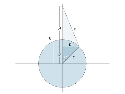
The problem when recreating the setup in 3D is that the piston’s y position is not linear connected to the rotation of the crankshaft. The piston will move at different speed during a full rotation. Start by opening the scene Piston_Engine.scn from this issues CD. Select the piston and press [Ctrl] + [K] to open its local transform PPG. Right click on the animation icon (the green divot) for the Y Pos and choose Expression Editor… from the menu. Since you know the length of the of the connecting rod, 11 units, and the radius of the crankshaft, 1.5 units, getting the pistons Y position is merely a task of putting your high school trigonometry knowledge into practice.

Side a is calculated by multiplying c (the radius of the crankshaft) with cosines alpha. Before you can determine side d you have to calculate side b, which is done by multiplying c (the radius of the crankshaft) with sinus alpha. Once b is known you can use the Pythagorean theorem,

d2 + b2 = e2 => d= square root(e2-b2)

The full height (h) is sum of a + d

Enter the following expression in the editing pane, press the Apply button and then close the Expression Editor.

1.5 * cos(Crankshaft.kine.local.rotz ) + sqrt( pow( 11, 2 ) - pow( 1.5 * sin(Crankshaft.kine.local.rotz ), 2 ) )

Aligning the connection rod can easily be done in the same manner as in the previous equation. Or you can simply parent the connection rod under the piston and make it point to the crankshaft by using a constraint. Select the ConnectionRod_Rotation, click the Parent button in the Main Command Panel and select the Piston with the middle mouse button to make it the child of the Piston. With the ConnectionRod_Rotation still selected, click the Constrain menu and choose Direction. Pick the Crankshaft_Center when prompted. In the Direction Constraint PPG –Y button to align the Connection Rod.

The project files used in this tutorial can be found at:
http://www.redi-vivus.com/Caffeineabuse/Piston_Engine.zip

Image 02
A quick revisit to your high school trigonometry lessons is just want the doctor has ordered.

Quick tip
All the transforms are evaluated in local space, so to move or reorient the piston simply parent all the objects under a null (or any other dummy object) and you’re good to go.

Read the full post>>

Single axis direction constraint

Image 01
While you can’t restrict the direction constraint to a single axis per se, using an extra object as a buffer will create the desired result.



As you’ve noticed there isn’t a one click solution to limit the direction constraint to a single axis. However there’s no need to despair as we’ve supplied you with two different methods to tackle the problem.

Open the scene Surveillance_Camera.scn from this issues DVD. The first method requires two null objects, one which can be moved in any direction and one that will be used for the actual direction constraint. Create a null object, name it Direction_Cns and move it somewhat in front of the surveillance camera. Create another null object, name it LookAt and move it in front of the camera as well. Press [Ctrl] + [K] to pen its Local Transforms PPG and click the Lock icon to pin it to the screen. Select the Direction_Cns object and press [Ctrl] + [K] to open its transform PPG as well. Click and drag the animation icon (the green divot) from the X Position in the LookAt PPG and drop it on the X Position animation icon in the Direction_Cns PPG. By dragging and dropping an animation icon from one parameter to another creates an equal expression, meaning the second parameter will match the exact same value as the first. Drag and drop the Z Position of the LookAt to the Z position of the Direction_Cns and close the PPG’s. Select the Camera_Orientation and from the Constrain menu choose Direction. Pick the Direction_Cns when prompted. Select and move the LookAt object to change the direction of the Surveillance_Camera. Save your scene under a new name.

The second method uses a somewhat different approach but has the same outcome. Open the Surveillance_Camera.scn again. Create a null object, name it Direction_Cns and position it straight above the camera. Create a second null, name it LookAt and position it in front of the camera. Select the Camera_Orientation object and from the Constrain menu choose Direction. When prompted, pick the Direction_Cns. Click the Y button in the Align Axis section of the Direction Cns PPG to correct the cameras orientation. Switch to the Up Vector tab. In the Optional Up Vector Control Object section, click the Pick New button and pick the LookAt object. Select Z as the Affected axis and close the PPG. While the direction is constrained to the Direction_Cns object, the added up vector gives you the final control of the cameras orientation. Select and move the LookAt object to change the direction of the Surveillance_Camera.

The project files used in this tutorial can be found at:
http://www.redi-vivus.com/Caffeineabuse/Direction_Constraint.zip

Image 02
The other way around it is to have the constraint pointing to a dummy object and then the up vector as the actual target for the direction.

Quick tip
In addition to naming convention it’s a good practice to use different colors and/or icons on your null objects. This way you can easily tell what objects does what by just looking at your scene.

Read the full post>>

Assigning different textures to the same geometry-instances in ICE

While you can’t assign different materials to the same geometry instances per se, you can use attributes from the pointclod to achieve the same result. Start by open the scene multiple_textures.scn from this issues CD. Select the PointCloud and press [Alt] + [9] to open an ICE Tree. With the pointcloud and the instanced geometry already in place, the only thing left to add is a random color. Get a Randomize Color by Gradient node and connect it to the Color input of the Emit from Surface node. Open the Randomize Color by Gradient PPG and change gradient to match the screenshot.

Select the can object and from the Get > Material menu choose Blinn to apply a material and then press [7] to open a Render Tree. While each particle has a random color assigned to it, the color information is not automatically passed on to the material. From the Attributes category get a Color node. Open its PPG and change the Attribute to Color.

From the Images Processing category get a RGBA Keyer and open its PPG. Set the both the Minimum and Maximum threshold color to R:0, G:1, B:0 (pure green). Set the Color if in rage to white (R:1 G:1 B:1), and the Color if outside range to black (R:0 G:0 B:0). This will create a mask where all the green particles will be output as white and everything else as black. Duplicate the RGBA Keyer node and change the Min and Max threshold color to pure blue (R:0, G:0, B:1).

In the Mixers category get a Mix 8 Colors node. Open its PPG and check the In Use checkbox for the Layer 2. Connect the Attribute Color node to the input of each of the RGBA keyer nodes. Connect the first RGBA keyer to the weight1 input of the Mix_8colors node and the second RGBA keyer to the weight2 input. Connect the Mix_8colors node to the diffuse and ambient input of the Blinn node. Add three image nodes, each with a separate texture, and connect the first to the base_color input of the Mix_8colors node, the second to the color1 input and the third image node to the color2 input. You’re now using three different textures on the same geometry-instances.

The project files used in this tutorial can be found at:
http://www.redi-vivus.com/Caffeineabuse/ICE_Textured_Instances.zip

Image 01
Using blocks of solid colors rather than the smooth gradient is a quick and efficient way to define random colors.
Image 02
The color information is then used in the Render Tree to assign a different texture to each of the colors defined in the gradient.

Quick tip
To change the balance between of the different colors (textures) simply change the markers position on the gradient.

Read the full post>>