The end of the blog…

So… The day have finally come when this blog will no longer get any updates. I want to thank everyone for all the emails, questions and comments I’ve received throughout the years. It’s been great to see so many of you enjoying the material on the blog and finding it useful.   

And now for the good news. I’m in the process of setting up my new site and have migrated all the material from the blog to its new home. The site is still very much in progress but please head to www.olamadsen.se to continue the caffeine abusing journey.

All the best and thanks for reading!

Read the full post>>

Example using the shockwave deformer

Here’s a quick example of deforming a water surface instead of a wall, as described in the tutorial.

http://caffeineabuse.blogspot.se/2014/07/build-your-own-shockwave-deformer-using.html

Read the full post>>

Build your own Shockwave deformer using ICE

The wave function

The shockwave will be constructed by two sets of waves - a somewhat smaller, condensed part followed by the larger more intense pulse. Even though a shockwave is an ideal candidate for simulation, it has a slight drawback - namely that it is simulated. Whenever you want to change a value or reposition the shockwave, you have to rewind and run the simulation again. An alternative approach is to do a bit of high school math. Don’t worry; it’s not as frightening as it sounds. The waveform is essentially nothing more than a sine wave; altered over time and its distance from the origin (technically, the equation actually uses the outer edge as the base for the calculation rather than the centre)  

The math

The animated sine wave consist of 3 building blocks. The first set of nodes uses the time attribute to change the values for each point over time and the distance from the deformation centre. The next set of nodes handles the frequency and the last set controls the amplitude or strength of the wave.

Open the Shockwave_start.scn scene from this issues CD. Select the Deform_Me geometry and press Alt + [9] to open an ICE Tree and from the Create menu choose ICE Tree. To make the following steps a bit easier to follow you’ll define all the parameters at the top of the tree and then simply getting those values as you need them as the Tree evolves. Get a Set Data node and connect it to Port1 of the ICETree. Get a Scalar node and connect it and then disconnect it to the New (Value) input of Set Data node 10 times to create 10 separate attributes. Open the Set Data PPG and enter the following attributes as the Reference. Use the number inside the parentheses as a starting point.  
self.Amplitude  (1)
self.SmallWaveRadius (11)
self.SmallWaveAmp (1)
self.SmallWaveLenght (4)
self.LargeWaveRadius (12)
self.LargeWaveAmp (2)
self.LargeWaveLenght (8)
self.Speed (0)
self.Distance (0)
self.Duration (40)

To set the speed of the wave you can get the current time in your scene and multiply it to increase or decrease the speed. So get a Current Time (which will return the time in seconds rather than frames) and a Multiply by Scalar node. Connect the Current Time to the Value input, set the factor to 10 and connect the Result output to the self.Speed input of the Set Data node. 
Rather than using the object’s actual centre point, you’ll use a separate null object and calculate the distance between each point of the geometry and the null. This enables you to reposition the null wherever you want the shockwave to start and the ICE tree will automatically take care of the rest. Get a Get Data node and enter Self.PointPosition as the Reference. Get another Get Data node and enter Impact_Center.kine.global.pos as the Reference. Get a Get Distance Between node and connect the self.PointPosition to its First input and the Impact_Center to the Second. Connect the Result output to the self.Distance input of the Set Data node.
While the Sin node will indeed give you a sine wave, it will be a static wave. In order to create an animated wave you need to change the value you feed into it over time, which is why you created the Speed attribute. Get a Get Data node and enter self.Speed as the Reference. Get another Get Data node and enter self.Distance as the Reference. Get a Subtract node and subtract the self.Distance from the self.Speed. The result of the subtraction will assign an incrementing value to each point over time and based on its distance from the centre. The value will however continue to increase to infinity, which will result in a continuous sine wave. An easy way to fix this is by clamping the output to 0. Get a Clamp node and connect the Result of the Subtraction to the Value input. Open the Clamp PPG and set the Limit 1 to 0 and the Limit 2 to a really high negative number, such as -1000000. 
The next step is to add control for the frequency (the number of waves). Get a Get Data node and enter self.SmallWaveLenght as the Reference. Get a Divide by Scalar node and connect the WaveLenght to the Value input. Open the PPG and set the Divide By to 360 and convert the output to Softimage units instead of degrees. Get another Divide by Scalar and connect the Clamp node to the Value input and Divide by Scalar to its Divided By input. Get a Sin node and connect the result of the division to its Value input. 
In addition to the frequency you also want to control the amplitude of the wave. Or the amplitude based on the waves distance to the center to be more precise. Get 3 Get Data nodes and enter self.Distance, self.Speed and self.SmallWaveRadius as their references. Get a Subtract node and subtract the self.Speed from the self.Distance. Get a Divide by Scalar and divide the result of the subtraction by the value output of the self.SmallWaveRadius. Get a Calmp node, set the Limit 1 to 0, Limit 2 to 1 and connect the result of the division to the Value input. The output of the Clamp node will output a decreasing value rather than increasing. To fix this, get a Subtract node, open the PPG and enter 1 as the First value. Connect the result of the Clamp node to the Second input. Since you’re gradually subtracting less from 1 for every frame, the output from the subtraction will obviously get closer to 1 over time. Get a Get Data node and enter self.SmallWaveAmp as the Reference. Get a Multiply by Scalar node and connect the WaveAmp to the Value input and the result from the Subtract node to the Factor. To bring the first wave together you just need to multiply the sine wave with the amplitude, so get another Multiply by Scalar node. Connect the Result of Sin node to the Value input and Result from the previous Multiply by Scalar node to its Factor input. 

The second wave

The math behind the large wave is identical to the first. The only thing you need to change is negating the sine wave and reversing the subtraction of self.Distance and self.Speed. Once this is done you can combine the 2 waves with a simple add node.

 With a few exceptions, the large wave uses the same math as the small wave. Select all the nodes constructing the small wave and press Ctrl + [C] and Ctrl [V] to copy and paste them. Replace all the ‘small’ with ‘large’ in the Get Data nodes (for example, self.SmallWaveLenght to self.LargeWaveLenght). Get a Negate node and intersect the connection from the Sin to the Multiply by Scalar node. You also need to reverse the subtraction of the self.Speed and the self.Distance, both for the frequency and for the amplitude. For the frequency the self.Speed should be subtracted from (Second input) the self.Distance (First input) and in for the amplitude the self.Distance should be subtracted from the self.Speed.

To add the two sets of waves together, get an Add node and connect the Result from the Multiply by Scalar from the small wave to Value1 and the Result from the large wave to Value2.
Get 2 Get Data nodes and enter self.Speed and self.Duration as their References. Get a Divide by Scalar and connect the self.Speed to the Value input and the self.Duration to the Divide By. Get an FCurve and connect the Result of the Division to its input. Open the FCurve PPG and add a keyframe with a value of 1 approximately at frame 0.2. Change the value of the keyframe at frame 1 to 0. This will scale the effect of the wave from 0 to 1 and back to 0 over its lifespan (which is defined by the duration attribute). Get a Multiply by Scalar and connect the Result of the Add node to the Value and the FCurve the Factor. 
The last step is to add a multiplication to scale the overall amplitude of the wave. Get a Get Data node and enter self.Amplitude as the Reference. Get a Multiply by Scalar and connect the Result from the previous multiplication to the Value and the self.Amplitude to the Factor.
The final step is to actually deform the geometry. Get a Get Data node and enter self.PointPosition as the Reference. This will return the X, Y and Z position for each of the points of the geometry. However, you’re only interested in changing the Y position (since the disc lies flat on the ground) so you need to separate the vectors. Get a 3D Vector to Scalar node and connect the self.PointPosition to its input. Get a Scalar to 3D Vector node and connect the X and Z output of the 3D Vector to Scalar to its corresponding inputs. Connect the Result output from the Multiply by Scalar node to the Y input of the Scalar to 3D Vector. Get a Set Data node and enter self.PointPosition as the Reference and connect the Scalar to 3D Vector to its input. Complete the ICE Tree by connect the Set Data node to the New (Port1)… input of the ICE Tree node.  

The complete ICE Tree

Read the full post>>

Future of the blog and completely unrelated cloud R&D

I haven’t been very active on the blog lately, which some of you may have noticed J I’ve got a just-about-finished tutorial describing how to create a ripple deformer in ICE with a “simple” equation. So, no simulation a fancy stuff like that. Just a couple of well-placed nodes J I also have a half-finished piece about creating a weightmap brush, with dispersion, decay etc, which I might finish if anyone asks for it.  In the meantime I’ll post some wip from a few projects I’ve been working on lately.

If you’re wondering about the future for the blog (given the depressing decision from Autodesk earlier this year) I can tell you that the blog will continue just as usual. Well, maybe not exactly as usual as I’m hoping to start adding content more frequently. In a not too foreseen future, the plan is to write articles and tutorials about another 3d application as well…  I am  very much in the learning process myself so I can’t say when I got any useful knowledge to pass on.

Read the full post>>

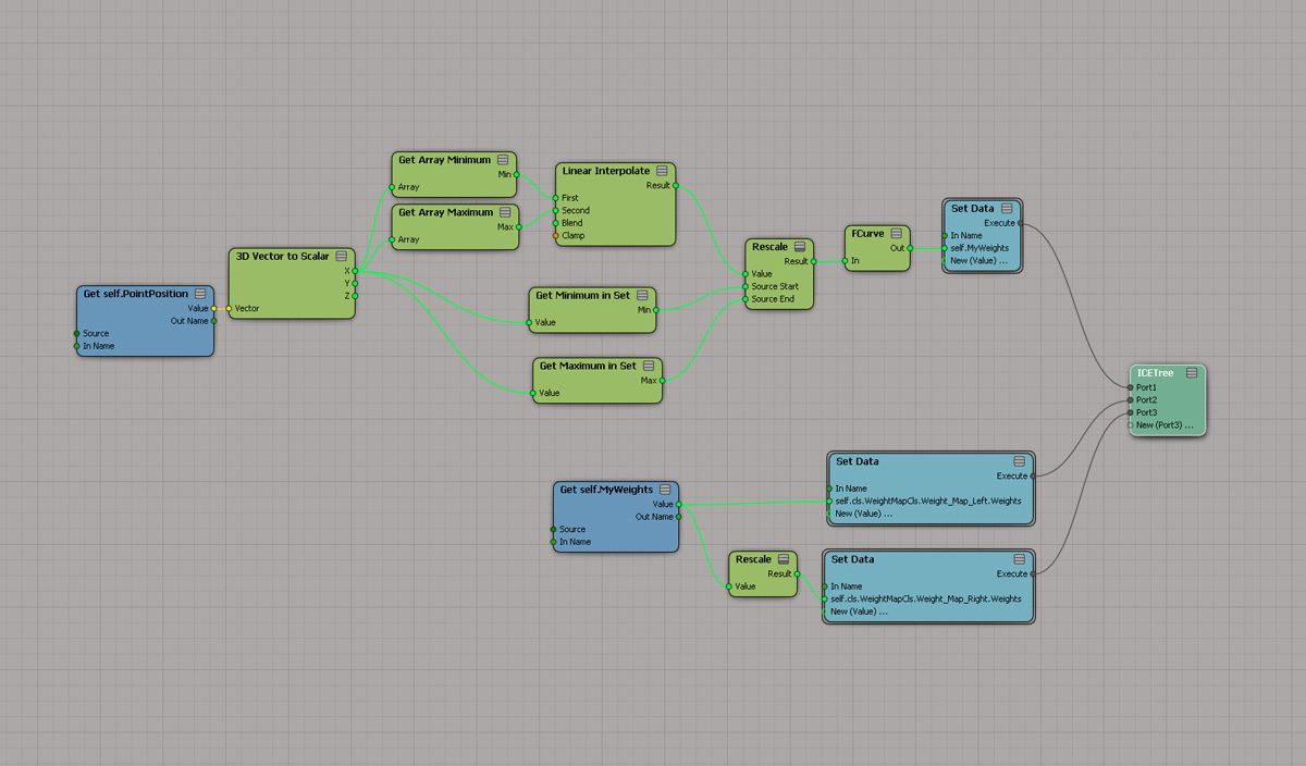
Automatic weightmaps for the left and right side of a head using ICE

Start by downloading and opening the scene ICE_Weightmaps.scn from https://dl.dropboxusercontent.com/u/3834689/CaffeineAbuse/LeftAndRight_Weightmap.zip. Before you can assign any weights use ICE you need an actual weightmap to assign them to. Select the Head object and from the Get > Property menu choose Weight Map. In the PPG, click the Rename button and rename it to Weight_Map_Left. Create a second WeightMap and rename it Weight_Map_Right. With the head still selected, press [Alt] + 9 to open an ICE Tree and from the Create menu choose ICE Tree. Get a Get Data node and enter self.PointPosition as the reference. To assign the proper weights to the weightmap you need to find where along the x-axis each of the points is located. If it’s higher a certain value (zero in this case) it’s part of the left side of the head, and if it’s lower (a negative number in this case) it’s part of the right side. While the get PointPosition node does get the position of the points on the geometry, it outputs them as a 3D vector (the X, Y and Z position and direction per point). So you’ll need to convert the 3D Vector to output the X, Y and Z component separately.

Since your calculating the distance between the points at the furthers left and right side, it doesn’t matter if the object is placed at the center of the scene or not. The distance between the minimum and maximum is always the same either way.

Get a 3D Vector to Scalar node and connect the Get PointPosition node to its input. By getting the position at the furthest right (maximum) and furthest left (minimum) and interpolate between the two you can assign a value to each point based on where it is located within that range. Sort of a percentage or gradient from furthest left to right if you will.

Get a Get Array Maximum and a Get Array Minimum node and connect the X output of 3D Vector to Scalar node to their respective Array input. Get a Linear Interpolate node and connect the Array Minimum to the First input and the Array Maximum to the Second input. The weights in the weightmap ranges from 0 to 1 so you need to rescale the current values which spans from -3.230 to 3.230 (their global x positions) to fit this range. Get a Rescale node and connect the Linear Interpolation node to its input. While you could enter the current minimum and maximum positions manually as the Source Start and End, your ICE Tree would only work on this specific model which really isn’t that useful. However, you already know the position of all the points so you can automatically get the highest and lowest number and plug that into the Rescale node. To do so, get a Get Maximum in Set and a Get Minimum in Set node and connect the X output of the 3D Vector to Scalar node to their respective Value inputs. Then connect the Maximum in Set to the Source End of the Rescale node and the Minimum in Set to the Source Start.

The FCurve node does not only enables you to create a smooth transition between the left and right weightmap, it also defines where each side start and ends. If your head is asymmetrical, simply nudge the keyframes to the left or right to aligned them with the geometry.

Get an FCurve node and connect the output of the Rescale node to its In input. Open the Fcurve PPG and select the Key at the left. Right-click on the Key and from the menu, choose Key Properties. Set the Frame value to 0.49. Click the Next Key button and change the Frame value to 0.51. This will create a smooth transition between the points of the left (with a value of 0) and right side (with a value of 1) of the head. Get a Set Data node, enter self.MyWeights as the reference and connect the output of the FCurve to its input. Then connect the Set Data node to the Port1 of the ICETree.

Get a Get Data node and enter self.MyWeights as the reference. Get a Set Data node, open its PPG and click the Explore button. Expand the tree in the explorer Head > Polygon Mesh > Clusters > WeightMap Cls > Weight_Map_Left and choose weights. Close the PPG and connect the Get self.MyWeights node the weights input of the Set Data node. Connect the Set Data node to the New (Port2)… input of the ICETree. To assign the weights for the right side weight map, all you have to do is to reverse the values. Get a Rescale node and connect the output of the self.MyWeights node to its Value input. Open the PPG and change the Target Start to 1 and Target End to 0. Get a Set Data node and repute the previous step but select the Weights for the Weight_Map_Right. Connect the Set Data node to New (Port3)… of the ICETree.

Quick tip
Whenever modifying or assign weights to weightmaps using ICE, you should always use a custom “buffer attribute” to do all your calculations. Then get the custom attribute and set the actual weights of the weightmap at the bottom of your ICETree.

Once you’re happy with the weightmaps it’s a good idea to freeze the geometry to avoid accidentally changing the weights. Please note that this will delete your ICE Tree so you might want to save the scene under a separate name for future reference.

Read the full post>>

Creating HDR environment maps from a 3D scene

Generating a HDR environment from your 3d scene is in fact not that much different from how you would go about in real life. The two most common options are to either shoot a chrome ball or to use multiple images to construct a spherical panorama. While there are 3rd party plugin which enables you to render the scene trough a spherical lens, you can just as easily create a virtual chrome ball to serve your needs.

The project files used in this tutorial can be found here: https://dl.dropboxusercontent.com/u/3834689/CaffeineAbuse/HDR_ProjectFiles.zip

Create the Chrome Ball 

Open the HDR_Environment.scn scene from this issues CD. Select the ChromeBall and from the Get > Material menu choose Constant. In the Constant Material PPG, switch to the Transparency/Reflection tab and set the Reflection Mix Color to pure white (R:1, G:1, B:1). This will turn the sphere into a perfect 100% reflective chrome ball. However, as the chrome ball is part of the scene it also means it will interfere with the lights, shadows, and so on, which probably is not what you want. 

Exclude the Chrome ball
With the chrome ball still selected, press [F3] to open a mini browser and click on the Visibility icon to open the PPG.  Uncheck the Shadow Caster and Shadow Receiver checkboxes.  While this will exclude it from casting and receiving shadows it still affects the final gathering in the scene. To avoid this, uncheck the Caster and Visible in Sampling attributes in the Final Gathering section of the PPG.

Generate the environment map
With the ball still selected, from the Get > Property menu choose Render Map.  In the Format section of the PPG, uncheck the Square checkbox and set the resolution to 1024 x 512. Click the New button next to the UV title and select Spherical to create a texture projection. Since you’re generating an HDR image you obviously need to use an image format supporting it. Change the output format to OpenEXR. By default reflection are disabled from the render map generation and while this is something you normally want it does counteract the sole purpose the chrome ball. In the Disable Surface Properties section, make sure uncheck the Reflection checkbox. Click the Regenerate Maps… button and you’re done.

Read the full post>>

Creating strands between two different objects

Once completed the following steps you’ve effectively generated strands between the objects, though they won’t show up in a rendered image as you haven’t  defined any size or shape yet. To do this simply get a Set Data node, right click on the Value Port of the node and choose Add Port After two times so you have three values. Open the PPG, enter self.Size as Reference and set the size to 0.1 or so. Enter self.Shape as Reference1 and choose Cylinder. To loft the shape along the strand rather than using individual shapes you’ll need to add one last attribute. Enter self.StrandDeform as Reference2, press enter and check the self.StrandDeform checkbox. Finally connect the Execute output of the Set Data node to the Port2 of the ICETree node.

The project files used in this tutorial can be found at: http://dl.dropbox.com/u/3834689/CaffeineAbuse/Strands_between_points.zip

Set the starting points

Open the scene Strands_between_points_Start.scn. From the Get > Primitive > Point Cloud menu choose Empty and press [Alt] + [9] to open an ICE Tree View. From the Create menu choose ICE Tree. Press [8] to open an Explorer and drag and drop the StartPosition grid into the ICE Tree. Get a get data node, open its PPG and enter .PointPosition as the Reference. Get another Get Data node and .kine.global as the Reference. Connect the Out Name output of the Get StartPosition node to In Name input of the two Get Data nodes. The point positions are stored in local space, meaning that you have to add the object’s transformation in order to retrieve the actual position of each point.  Get a Multiply Vector by Matrix node and connect the Value output of Get .PointPosition to the Vector input and the Value output .kine.global node to the Matrix input. 

The end point

Get an Add Point node and connect the Result output of the Multiply Vector by Matrix node to the Positions1 input. Then connect the Add output of the Add Point node to the Port1 of the ICETree node. This will create a point at each of the grids vertices and will be used to create the strands. Get a Build Linearly Interpolated Array node and a Get Data node. Enter Self.PointPosition as the Reference and connect the Value output to the Start input of the Build Array node. Open an Explorer and drag and drop the EndPosition grid into the ICE Tree.  Repeat the previous step and connect the PointPosition, kine.global and Multiply Vector by Matrix nodes.

Create the strands
While you’ve just defined the end position for the strands you can’t feed this information directly into Build Array node because the point positions derive from different component types (points vs. vertices).  To fix this, get a Switch Context node and connect Multiply Vector by Matrix node to its Value input. Then connect the Result of the Switch Context to the End Value of the Build Array node. Get a Set Data node, enter self.StrandPosition as the Reference and connect the Result of the Build Array node to the input. Connect the Execute output of the Set Data node to the On Creation1 input of the Add Point node.

Read the full post>>

Using an animated map to define particle goals in Softimage

There’s a slight difference depending on what map you’re using. A texture map is essentially an image file connected to an object, and as such you need to tell ICE what to do with this information before you can make use of it. First you need to convert the RGB color of the image to a scalar value and store this information as a custom attribute. Weightmaps on the other hand are already stored as scalar values, and as such you can skip the first step and use its Weights attribute directly in step 2. Start by opening the scene Goal_using_TextureMap.scn. 

The project files used in this tutorial can be found at:http://dl.dropbox.com/u/3834689/CaffeineAbuse/GoalLocation_using_AnimatedMaps.zip

Create a custom goal attribute
Select the Goal_Object and press [Alt] + [9] to open an ICE Tree. From the Create menu choose ICE Tree. Get a Get Data node, open its PPG and enter Self.NodeLocation as the reference. Get another Get Data node and enter Texture_Map as the reference. Connect the Value output of the Get Self.NodeLocation to the Source input. Get a Color to Brightness node and connect the value of the Get Texture_Map node to its Color input. Get a Set Data node and enter Self.GoalTextureMap as the reference and connect the Brightness output of the Color to Brightness node to the input. Connect the Set Data node to Port1 of the ICE Tree.

Set the GoalLocation

Select the pointcloud and update the ICE Tree view. Get a Get Data node and enter Goal_Object as the reference. Get a Get Geometry Sample node and connect the Value output of the Get Goal_Object node to the Geometry Input and then open its PPG. This node enables you to filter which part of the surface to use as the goal by extracting the weights from either the weightmap or the custom attribute created for the texture map.  Click the Explore button in the filter section of the PPG, expand the Input> Polygon Mesh tree and select the GoalTextureMap attribute. 

Move towards goal

Get a Set Data node and enter Self.GoalLocation as the reference.  Connect the Samples output of the Get Geometry Sample node to Self.GoalLocation input of the Set Data node. Connect the Set Data node to the Execute on Emit1 input of the Emit from Geometry. This will define the goal for each particle as it’s born. Once defined, you’ll use another node to actually move them there. Get a Move Towards Goal node and connect it to the Execute1 input of the Simulation Root node. Playback the animation and you’re done.

Read the full post>>

Wall of lights - How to set up a wall of animated light bulbs

The perhaps most intuitive way to create different patterns for the lights switching on and off is by using a texture map, which in turn controls the lights based on the lightness of the images.

Nine out of ten times you’re overegging the pudding by adding actual light source to the setup as you most likely could get away with a using really bright material on the object. But there is that one time you do need it, and this apparently is it.

Start by opening the scene Light_Wall.scn from this issues CD. There are several ways you can animate the lights switching on and off, but the perhaps most intuitive is by using an image sequence. Select the Wall object and from the Get > Property > Texture Map menu choose Texture Map. In the Clip section of the PPG, click the New button  and choose New From File. In the Browser, select the LightSwitch.pic sequence from the Pictures folder and click OK. Select the Texture_Projection in the UV Property section and then close the PPG.

From the Get > Primitive > Point Cloud menu choose Empty and press [Alt] + [9] to open an ICE Tree. From the Create menu choose ICE Tree. Press [8] to open an Explorer and drag and drop the Wall object into the ICE Tree. Get a Get Data node and connect the Out Name output of the Wall node to its In Name input. Open its Property Page (PPG) and enter PolygonPosition as the reference. This will get the centre of each of the polygons of the wall object, but as the object itself is rotated you’ll also need to add the global rotation. This is done by multiplying the polygons position with the objects global matrix. Get a Get Data node and enter kine.global as the reference and connect the Name output of the Get Wall node to the In Name input. Then get a Multiply Vector by Matrix node and connect the Value output of the Get PolygonPosition node to the Vector input and Value output of the kine.global to the Matrix input. Get an Add Point node and connect the Result output of the Multiply Vector by Matrix to the Positions1 input. Connect the Add output of the Add Point node to the Port1 of the ICE tree. Get a Set Data node, enter Self.Size as the reference and then enter 1 as the Size. Connect the Execute output of the Set Data node to the Port2 input of the ICE Tree.

Get a Get Closets Location node and connect the Value output of the Get Wall node to its Geometry input. The location you want to get is the location closest to each point so get a Get Data node, enter Self.PointPosition as the reference and connect it to the Position input of the Get Closest Location node. Then connect the Value output of the Wall node to the Geometry input. Get a Get Data node, enter Texture_Map as the reference and connect the Location output of the Get Closest Location to its Source input. Get a Color to Brightness node and connect the Color output of the Get_Texture to its Color input.

Get an Instance Shape node and open its PPG. Click on the Explore button and select the Light_ Bulbs group. Change the Hierarchy Mode to Object and Children. The Index value controls which object/hierarchy to be used. If the lightness value of the texture map is less than 0.5, the light should be off and the light bulb hierarchy with Index 0 should be used. If the lightness is higher than 0.5 the light should be switched on and the hierarchy with the added point light (index 1) should be used instead. Get a Round node and connect the Brightness output of Color to Brightness to its Value input. Then connect the Integer output of the Round node to the Index input of the Instance Shape. Connect the Shape output of the Instance Shape to the New(Value) input of the Set Data node. Open the PPG and enter Self.Shape as Reference1.

While the points are in the right locations they are facing the wrong direction. To fix this, you can get the orientation of each of the polygons and then use that data to set the orientation of the points. Get a Get Data node and enter PolygonRefFrame as the reference. Get a Matrix to SRT node and connect the Value output of the PolygonRefFrame to the Matrix input. Connect the Rotation output of the Matrix to SRT to the New(Value) input of the Set Data node. Open the PPG and enter Self.Orientation as Reference2.

Using actual light sources will cost you when it’s time to render and in most scenarios you won’t be able to tell the difference from using a really bright material on the object instead.

The project files used in this tutorial can be found at: http://dl.dropbox.com/u/3834689/CaffeineAbuse/Wall_of_Lights.zip

Quick tip
To add color to the lights you can add a second texture map using a different image sequence. Use the same approach as for the first map, but connect the Value output of the Texture_Map directly to a Self.Color input on the Set Data node. Then add a Color_Attribute node (with the Attribute set to Color) to the light’s Render Tree and connect it to the color input of the soft_light shader.  

Read the full post>>

Rigging an accordion lamp

The distinctive design of the accordion lamp may look simple to rig, but don’t be fooled. As the lamp expands or contract the joints at each end of the arms moves in a circular motion, rendering the standard constrains useless.

The accordion lamp consists of a series of individual arms which are mounted in pairs creating an X-Shape. Rotating any of the arms will cause all arms to rotate which either expand or contract the lamp. Start by open the scene Accordion_Lamp.scn. The scene consists of a number of null objects and the arms, which are parented under the null representing their respective centre joint.  

Select the Center1 null, press [Ctrl] + [K] to open its Local Transform PPG. Right-click on the animation icon (the green divot) for the X Axis Position and choose Set Expression... The arms are distributed linearly between the base (the part attached to the wall mount) and the lamp and since there are 4 pairs we know that the first joint should be located at 1/8 of the distance to the End null. In the Editing Pane of the Expression Editor, enter 1/8*End.kine.local.posx and click the Apply button. Open the Local Transform PPG for the Center2, right-click on animation icon for the X Axis and enter 3/8*End.kine.local.posx as expression. Repeat the procedure for the Center3 (5/8*End.kine.local.posx) and Center4 (7/8*End.kine.local.posx) nulls.

To determine the Y position of the top joint of the arm (the arm’s rotation) you need another null object, but foremost you need Pythagorean Theorem. The theorem states that if you know the length of two sides of a right-angled triangle you can calculate the length of the third side (a² + b² = c²). The length of side a is the distance between the wall mount and the Center1 null. The length of side b is the distance between the center joint and the top joint of the arm, in this case 3.5 units. Select the Top_Joint1 null and open its Local Transform PPG. Right-click on the animation icon for the Y Position and choose Set Expression… Enter sqrt( pow( 3.5, 2 ) - pow( Center1.kine.global.posx, 2 )) in the editing pane and click the Apply button to apply the expression. 

For the Top_Joint2 you must not only calculate the Y position but also the X position as this will change as the lamp expand or contract. Open the Top_Joint2’s Transform PPG and apply an expression to the X position. The joint will always be located at the middle of the Center1 and Center2 nulls, which you can calculate by adding their X positions and then divide it by 2. Enter ( Center1.kine.local.posx + Center2.kine.local.posx ) / 2 and click the Apply button. Close the Expression Editor and apply an expression to the Y Position. The length of side b is still 3.5 in this triangle, but side a equals half the distance between Center1 and Center2. Enter sqrt( pow( 3.5, 2 ) - pow( ( ctr_dist( Center1.kine.global.pos, Center2.kine.global.pos ) / 2 ), 2 ) ) and click the Apply button.

Select the Arm01 and from the Main Command Panel > Constrain menu choose Direction and pick the TopJoint1 null. Select Arm02, apply a Direction constraint but this time pick the TopJoint2 null. Repeat the last two steps for the Top_Joint3 and 4 and their respective arms.

The project files used in this tutorial can be found at: http://dl.dropbox.com/u/3834689/CaffeineAbuse/AccordionLampRig.zip

Looking at the accordion lamp you’ll see that it’s in fact made by multiple triangles. Pythagorean Theorem states that if you know the length of two sides of a right-angled triangle you can calculate the length of the third side.

Quick tip

Once you’ve calculated the rotation for the first arm, you’ve essentially calculated the rotation for all arms. Rather than using the theorem and contains you can simply add an equal expression to the subsequent arms Z rotation, Arm01.kine.local.rotz to the odd arms and –Arm1.kine.local.rotz to the even.

Read the full post>>

Using render channels in Softimage

The typical use of render channels is to render the scenes components, such as ambience/diffuse, reflection or motion vectors into individual images. As most of these components are calculated individually by Mental Ray anyway they're not going to affect the time needed to render the image. In addition, channels can be used to render partial or multiple render trees, adding ambient occlusion, outputting mattes or any other type of information within a single pass. In this case however, you won't get them for free. 

The project files used in this tutorial can be found at:  http://dl.dropbox.com/u/3834689/CaffeineAbuse/Render_Channels.zip

01 Adding the channel
Open the scene Render_Channels.scn from this issues CD. Select the Jigsaw_Piece_01 object and press [7] to open a Render Tree. Get a  Store Color in Channel node and open its PPG. The Store Color in Channel can be inserted anywhere in your render tree to store a specific part of the tree to custom render channel. But it can also be used to store information that is not part of the actual material. In the Render Channel section of the PPG, expand the drop down menu and choose the AmbOcc Channel. Get an Ambient Occlusion node and connect it to the Input of the Store Color in Channel node.

02 Store the information
Get another Store Color in Channel node. Open the PPG and click the Add button and enter RGB_Matte as the Render Channel Name and click OK. Set the Input color to pure red.  Get a Color4_Passthrough node and connect the Blinn node to its Input. Connect the Result output of the Color4_Passthrough node to the Surface Input of the Material node. The passtrough node acts as a hub and allows you to store as many channels as you like. Open its PPG and click the Add button twice to add 2 channels. Close the PPG and connect each of the Store Color in Channel node to the Channels > Item inputs.  

03 Render the Channels
Repeat the procedure for the other Jigsaw pieces, but set the Color of the RGB_Matte channel to pure blue for the second piece, pure green for the third and pure black for the forth. Close the Render Tree. From the Render > Render menu, choose Render Manager... In the Render Channels Output section, click the Add button. Select the AmbOcc channel in the Render Channel drop down menu and click OK. Click the Add button again, select the RGB_Matte channel and click OK. Your pass is now ready for rendering, so click the Render button and choose Render Current Frame.

Quick tip
It's important to note that if you need to re-render one of the channels, you will need to re-render the entire pass which may take considerable longer than if you where using separate passes. So contemplate which is the most beneficial in any given scenario. 

Read the full post>>

Shape blending in ICE using an image sequence

Since you'll be using ICE to control the blend of the shape keys, make sure there aren't any shape tracks added to the Animation Mixer and delete the Cluster Shape Combiner operator in the Shape Modeling stack of the object.
Open the scene Blend_Shape_Using_TextureMap.scn. Select the Can object  and from the Get > Property > Texture Map menu choose Texture Map. In the Clip section of the PPG, click the New button and choose New From file from the popup menu. Select the Gradient_Mask.jpg sequence and click OK to load the images. Select the Texture_Projection in the UV Property.

With the Can still selected, press [Alt]+[9] to open an ICE Tree view. From the Create menu choose ICE Tree. Get a Get Data node, open its PPG and enter Self.PointPosition as the Reference. Get another Get Data node, open its PPG and click the Explore button. Expand the Can > Polygon Mesh > Clusters > Can_ShapeKey > Can_ShapeKey branch of the tree and select the positions element. What you want to do is interpolate or blend between the objects current point position and the positions of the shape key. Get a Linear Interpolate node and connect the Value output of Get Self.PointPosition node to its First input.

The shape key does not store the actual point position of the shape,  but the points' change in position in relation to the initial mesh. To get  the actual positions you need to add the shape to the current point position. Get an Add note and connect the Self.PointPosition to the Value1 input of the Add node and the Get Can.cls.Can_ShapeKey.Can_ShapeKey.positions to the Value2 input. Connect the Result of the Add node to the Second input of the Linear Interpolate node.  Get a Set Data node and enter Self.PointPosition as the Reference in the PPG. Connect the Result output of the Linear Interpolate node to the Self.PointPosition input of the Set Data node. Connect the Set Data node to the Port1 input of the ICETree node.

The blend value of the Liner Interpolation node controls how much influence each of 2 input values will have. A value of 0 means the second value of the Linear Interpolation node will have 0 affect which results in the first value having full affect. With the blend value set to 1, the opposite is true and the second input will have full affect and the first input 0. Instead of setting the blend value for the entire mesh at once, you can set  it per point based on the RGB value of an image sequence. Get a Get Point Texture Map Color node and a Color to Brightness node.  The Color to Brightness node converts the RGB value of the image to a scalar value which in can then be used to control the blending of the Linear Interpolation. Connect the Value output of the Get Point Texture Map Color node to the Color input of the Color to Brightness node. Connect the Brightness output of the Color to Brightness node to the Blend input of the Linear Interpolate node.

The project files used in this tutorial can be found at:  http://dl.dropbox.com/u/3834689/CaffeineAbuse/ShapeBlendingWithICE.zip

While you typically want to set the blend value between zero and one, you can use values above 1 to amplify the affect or negative values to inverse it.

Quick tip
If you want to blend between more than 2 shapes you can use the Blend node instead. Note that the blend node will output the weighted sum of all the inputs, so if you increase the weight of one input you'll need to equally decrease the weight of the other inputs to avoid double transformation. 

Read the full post>>

Turbulize the position of a locator with ICE kinematics

Controlling the scale, transformation or rotation (SRT) of an object with ICE isn't any different from doing the same when dealing with point or "particles". The thing you need to keep in mind though is how you set the data. While you can read any of the SRT properties of an object you can't set the individual X,Y or Z transforms directly nor their local transform values. In order to set any of the transform values you need to set the whole global transform matrix. Note that this is merely a structural thing and does not affect what you can and cannot do with an object’s SRT. 

01 Creating the scene

Get a Sphere (From the Get > Primitive > Polygon Mesh menu) and a Null object (From the Get > Primitive menu). The null object serves as a place holder for your ICE Tree. Select the Null object and press [Alt] + [9] to open an ICE Tree view. Get a Get Data node, open its PPG and enter sphere.kine.global as the Reference. In order to change the individual components of the SRT matrix you first need to deconstruct the matrix, make the modifications to the respective components, and then put the matrix back together. Get a Matrix to SRT node and connect the Value output of the sphere.kine.global node to its Matrix input. Get a SRT to Matrix node and connect the Scaling and Translation output of the Matrix to SRT to its corresponding input.

02 Deconstructing the Matrix

Get a 3D Vector to Scalar node and connect the Translation output of the Matrix to SRT to its Vector input. Get a 3D Vector node, a Turbulence node and a Multiply node. Connect the 3D Vector to the Position input of the Turbulence node and the Turbulence to the Value1 input of the Multiply node. Get a Add node and connect the Y output of the 3D Vector to Scalar to its Value1 input. Connect the Multiply node to the Value2 input of the Add node. Open the Turbulence PPG and lower the Time Frequency to 0.5 or so. This will control the speed of the turbulence. The Multiply node controls the strength of the turbulence. Open the PPG and set the Value2 to 20

 

03 Put the Matrix back together.

By using the Add node, the turbulence will be added on top of the Sphere's Y translation rather than completely replacing it. Get a Scalar to 3D Vector and connect the X and Z output of the 3D Vector to Scalar node to its corresponding inputs. Connect the Result output of the Add node to the Y input. Connect the Vector output of the Scalar to 3D Vector node to the Translation input of the SRT to Matrix node. Get a Set Data node, open its PPG and enter sphere.kine.global as the reference. Connect the Matrix output of the SRT to Matrix node to the sphere.kine.global input of the Set Data node. Connect the Execute output of the Set Data node to the port1 of the ICETree node. 

The project files used in this tutorial can be found at:http://dl.dropbox.com/u/3834689/CaffeineAbuse/ICE_Kinematic_Turbulence.zip

Read the full post>>